# Install (if needed)
# install.packages("VIM")
library(VIM)

# Aggregation plot of missingness
aggr(airquality, numbers = TRUE, prop = FALSE)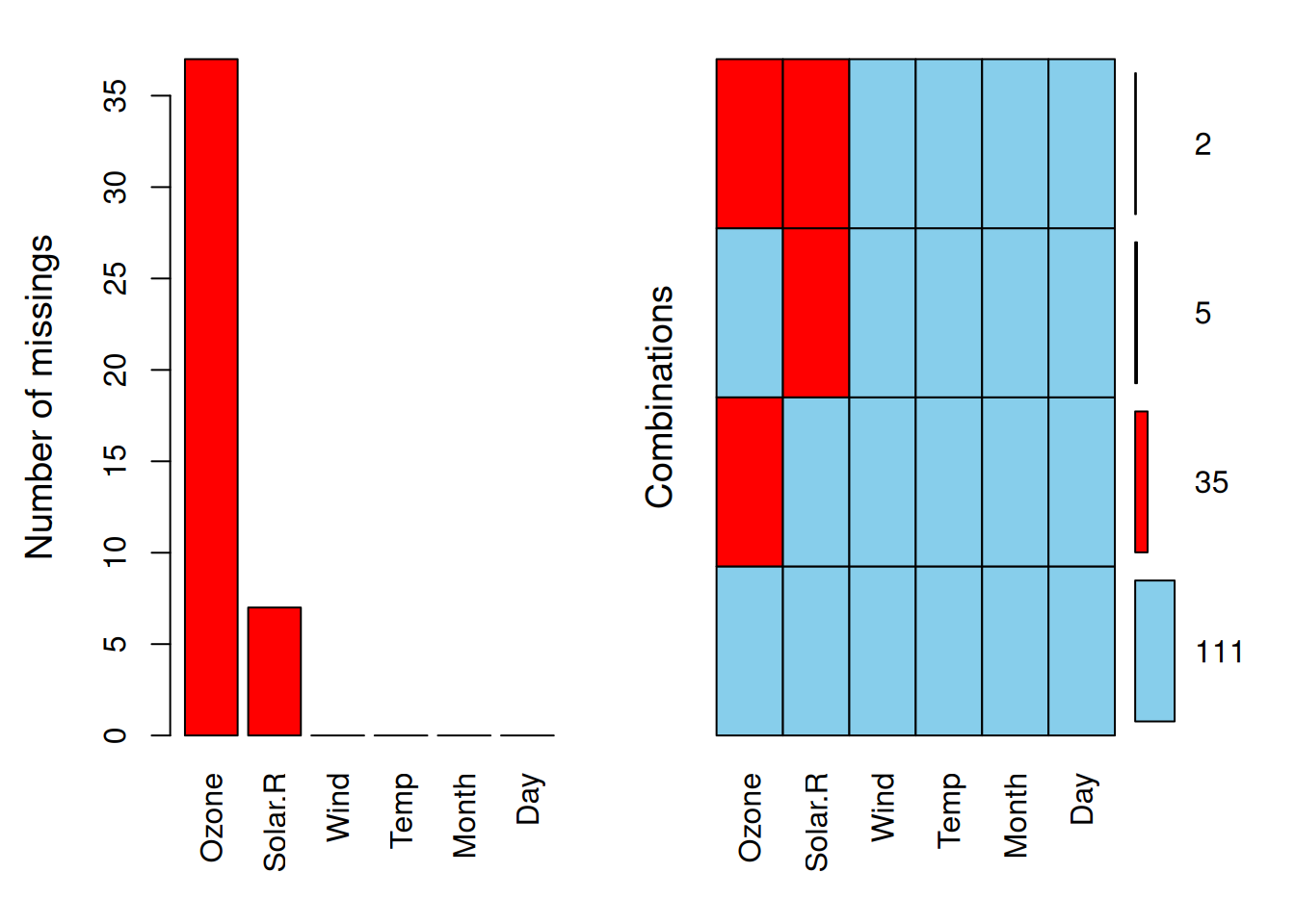
Missing values happen when data for an observation is not recorded. This can occur if, for example, a participant drops out of a study, a machine fails, someone skips a survey question, or a recording error is made.
Missing data are usually shown as an empty cell, a \(.\) (dot), or a \(*\) (asterisk). Invalid entries – like text in a numeric column or a N/A error – are also treated as missing.
Sometimes older datasets use numbers like \(99999\) to mark missing data. In such cases, replace them with a proper missing value indicator before analysis.
The missing values can take the form of blank cells, null values or special symbols like NA, NaN or “unknown”
Handeling missing values is essential for accurate and reliable analysis. Key reasons include:
Better Model Accuracy: Fixing missing data improves predictions and model performance.
Maintained Sample Size: Imputation or careful removal keeps more data available for analysis.
Reduced Bias: Proper handeling prevents distorted or misleading results.
Stronger Decisions: Clean data leads to more confident and trustworthy conclusions.
Missing data can create problems such as
Smaller Sample Size: Removing rows with missing values reduces data and reliability.
Biased Results: Non-random missing data can lead to false conclusions.
Limited Analysis: Many methods can not handle missing data, restricting analysis options.
Data may be missing due to:
Technical issues: Equipment failure or data transfer errors.
Human errors: Mistakes in entry or recording.
Privacy concerns: Withholding sensitice information.
Processing problems: Errors during data preparation or transformation.
Before handling missing values, it is IMPORTANT to understand why they are missing – this is part of what we can call data intuition, or the ability to look closely at your data and reason about what is happening.
Ask yourself this key question:
Is the value missing because it was recorded, or because it does not exist?
If it does not exist (for example, the height of the oldest child of someone who does not have any children), it does not make sense to fill it in – keep it as NaN.
If it was not recorded (for example, a measurement that someone forgot to take), you may estimate it using other available data. This process is called imputation.
Undertanding the reason behind missing values you decide whether to leave them as missing or fill them in intelligently.
Let us start with an example, the airquality dataset, which records daily air quality measurements in New York (1973).
It has missing values in Ozone and Solar.R columns.
Also, we can cofirm this using anyNA().
TRUE indicates a presence of missing values in our data.
There are some libraries that can help us visualize missing data patterns, such as naniar, VIM, and mice
# Install (if needed)
# install.packages("VIM")
library(VIM)
# Aggregation plot of missingness
aggr(airquality, numbers = TRUE, prop = FALSE)
Sometimes, we expect a value in our dataset, but it is not there. For example, a survey respondent may skip a question, or a sensor may fail to record a measurement, or a file got lost. These are missing values. But not all missing values happen for the same reason – and the reason matters, because it affects how we should handle them.
Think of this as:
The data went missing by accident.
This missingness has nothing to do with any variable in your dataset. It is just a bad luck – like someone spilled coffee on some forms or a sensor failed. Everyone had an equal chance of having missing data.
For example, a few lab samples are lost because a fridge broke. This has nothing to do with the people or the measurements. ::: callout-important If data are MCAR, your analysis will still be fair and unbiased, even if you remove those cases. :::
Think of this as:
The data is missing for a reason we know about.
This missingness is related to other variables that we have data for. But it is not related to the value that is missing itself.
For example, you ask people about their income, and you notice that younger people are less likely to answer. So the missingness depends on age (which you know), not on income itself.
You can fix this by using the other variables (like age) to estimate or impute the missing ones.
Think of this as:
The data is missing because of the value itself.
The missingness is related to the thing that is missing or maybe you do not know the reason at all.
For example, some people do not report their weight because they feel uncomfortable about it – so the missingness depends on weight itself.
This is the hardes case – because we can not fix it easily. You may need special models or collect more data.
For each of situation below, decide whether the missing data are: (A) Missing Completly at Random (MCAR), (B) Missing at Random (MAR), or (C) Missing Not at Random (MNAR).
Question 1 During data entry, some survey responses were lost because the computer crashed before saving. What type of missingness is this?
Question 2 In a health survey, people with higher income are less likely to reveal their income, but everyone answered all other questions. What type of missingness is this?
Question 3 A researcher measures blood pressure, but the cuff sometimes fails to inflate due to a machine error, affecting random participants. What type of missingness is this?
Question 4 In a questionnaire about mental health, people with higher levels of stress are more likely to skip the “stress level” question. What type of missingness is this?
Question 5 Some students forgot to write their age, but we notice that older students tend to complete the survey more carefully and rarely miss answers. What type of missingness is this?
Question 6 A dataset on patient weight is missing for extremely obese individuals because the hospital’s scale cannot record weights above \(200\) kg. What type of missingness is this?
Question 7 An old version of a form did not include the “education level” question, but the new form does. What type of missingness is this?
Question 8 After a customer service call, customers are asked to rate their experience with the representative. Some customers give feedback, and others do not. Assume that the decision to give feedback is completely random, with no connection to the customer’s experience or any other factor. What type of missing data best describes the missing values in the feedback column?
Question 9 In a dermatology clinic, a survey is conducted asking patients about their gender and their skincare routine. It turns out that women are more likely to respond, while men often skip the question. What type of missing data best describes the missing values in the skincare routine column?
Solution.
Question 1: MCAR – Data lost by accident; unrelated to any variable.
Question 2: MNAR – Missingness depends on the income value itself.
Question 3: MCAR – Random machine fault.
Question 4: MNAR – Missingness depends on stress level itself.
Question 5: MAR – Missingness depends on another variable (age).
Question 6: MNAR – Missing because of the actual value (very high weight).
Question 7: MAR – Missingness linked to the form version (observed variable). Question 8 MCAR – The missing feedback is unrelated to any variable — it is random. Question 9 MAR – The missingness is related to another variable (gender) that is observed, not to the skincare routine itself.
Once we identify that some data are missing, we need to decide how to deal with them. The goal is to reduce bias and make sure our analysis remains reliable. The best method depends on why the data are missing (MCAR, MAR, or MNAR), how much is missing, and what type of variable we are dealing with (numeric, categorical, or time-series)
If possible, the best option is to go back and collect the missing data – by recontacting participants, checking logs, or re-running measurements.
This method is best for small and important datasets but it is time-consuming or impossible after data collection.
This means removing the rows or columns that contain missing values.
If a column has too many missing values (for example, more than \(70\)-\(80\%\) of the entries are NA), it may be better to remove it completely.
data <- data[, colSums(is.na(data)) < 0.8 * nrow(data)]

# or equivalently
data <- data[, colMeans(is.na(data)) < 0.8]We use this method when most values in a column are missing.
Using this method results in loss in information
You can also remove entire rows that contain at least one missing value. This is simple but can lead to data loss if missingness is common.
Listwise deletion (also called case deletion) is the default behaviour in R. This methods removes all rows (cases) that contain at least one missing value, regardless of which variable it occues in. For example,
linear_model <- lm(Ozone ~ Solar.R, data = airquality)
summary(linear_model)
Call:
lm(formula = Ozone ~ Solar.R, data = airquality)

Residuals:
    Min      1Q  Median      3Q     Max
-48.292 -21.361  -8.864  16.373 119.136

Coefficients:
            Estimate Std. Error t value Pr(>|t|)
(Intercept) 18.59873    6.74790   2.756 0.006856 **
Solar.R      0.12717    0.03278   3.880 0.000179 ***
---
Signif. codes:  0 '***' 0.001 '**' 0.01 '*' 0.05 '.' 0.1 ' ' 1

Residual standard error: 31.33 on 109 degrees of freedom
  (42 observations deleted due to missingness)
Multiple R-squared:  0.1213,    Adjusted R-squared:  0.1133
F-statistic: 15.05 on 1 and 109 DF,  p-value: 0.0001793
If you check the model output, R shows at the bottom something like:
42 observations deleted due to missingnessThis message means R autoamtically exculded rows with any missing values before fitting the model.
You can also perform listwise deletion manually:
data_without_missing <- na.omit(data)Another way is to use only complete cases (rows without any NA).
data_without_missing <- data[complete.cases(data),]Use this method when only a few rows have missing values.
Avoid this method when many rows have missing values since you may lose too much data.
Listwise deletion gives valid (unbiased) results only when the missing data are MCAR and the amount of missing data is small.
Instead of deleting a whole row, each pair of variables is analyzed using all available data for that pair.
Here, rows are only excluded when data are missing for the specific variables being compared.
In R, some correlation functions support this:
cor(data, use = 'pairwise.complete.obs')Although using this method uses more data and does not discard rows entirely, different analyses may use different subsets of data which can make results inconsistent or hard to reproduce.
This means replacing missing values with estimated values. There are many ways to do this – from simple to advanced.
replace misisng values with a fixed number (e.g., \(0\) or “unknown”)
Replace missing values with the column mean or median (for numeric data), median or mode (for categorical).
If you want to impute multiple numeric columns at once (for example, using the mean), you can use across() like this
This automatically fills missing values with mean of each numeric column.
Using this method reduces variability and can distort relationships
Group-wise Mean/Median Imputations Sometimes, imputing within groups makes more sense.
For instance, if passengers of similar class share similar ages, we can use:
library(dplyr)
data <- data %>%
  group_by(Class) %>%
  mutate(Age = if_else(is.na(Age), mean(Age, na.rm = TRUE), Age))%>%
  ungroup()
Use this when a grouping variable logically explains variation in missing data.
For categorical variabels, replace missing values with the most frequent category or, if many values are missing, a new category such as “unknown”. For example, in a dataset for the variable Gender, we can have
# replace NA with the most common category
mode_value <- names(sort(table(data$Gender), decreading = TRUE))[1]
data$Gender[is.na(data$Gender)] <- mode_value

# Or add a new category
data$Gender <- ifelse(is.na(data$Gender), "unknown", data$Gender)For time-series data, you can fill missing values using the previous or next observed value.
# install.packages("zoo")

library(zoo)

# Forward fill
data$Temperature <- na.locf(data$Temperatue, fromLast = FALSE)

# Backward fill
data$Temperature <- na.locf(data$Temperatue, fromLast = TRUE)
Use this method when data are sequential and values change smoothly over time.
Interpolation estimates missing values based on neighboring points – ideal for regularly spaced time-series.
# install.packages("imputeTS")

library(imputeTS)

data$Temperature <- na_interpolation(data$Temperature, option = "linear")
Use this method when values follow a continues trend (e.g., temperature, stock prices).
Some models can handle missing data automatically, without imputation.
For example,
model <- lm(Ozone ~ Wind + Temp + Solar.R, data = airquality)
pred <- predict(model, newdata = airquality)
airquality[is.na(airquality$Ozone)] <- pred[is.na(airquality$Ozone)]# install.packages("VIM")
library(VIM)
data_kNN <- kNN(airquality, k = 5)Use this method when variables have meaningful similarity structure. It is important to note that this method is computationally expensive for large datasets.
Dataset1 airquality dataset
data("airquality")The dataset records daily air quality measurements in New York (1973). It has missing values in Ozone and Solar.R columns.
Question 1:
Examine the distribution of Ozone and Solar.R columns. Are they normally distributed or skewed? (Hint: use summary(), histogram or boxplot)
Based on the shape of the distribution, decide whether to use mean or median imputation for each column.
Replace missing values in Ozone and Solar.R using your chosen method with dplyr.
Question 2:
Month (i.e., replace missing values with the mean or median within each month), whichever you think is more appropriate.** Dataset2** nhanes dataset from mice package
# install.packages("mice")
library(mice)
data("nhanes")
Question 1:
Explore the nhanes dataset to identify columns with missing values. Use summary() and md.pattern() from the mice package.
Choose a categorical column with missing value and impute missing values using mode.