7 Outlier Detection: Understading and Handling

7.1 Definition and Causes of Outliers

7.1.1 What are outliers?

An outlier is an observation that differs significantly from other observations.

Outliers may appear as unusually large or small values and are sometimes referred to as anomalies.

The ouliers can represent important, rare, or faulty observations. Therefore, detecting and interpreting outliers should always involve contextual and domain-specific judgment — not just automated rules.

Note

An observation must always be compared to other observations made on the same phenomenon before actually calling it an outlier. Indeed, someone who is 2 meters tall will most likely be considered an outlier compared to the general population, but that same person may not be considered an outlier if we measured the height of basketball players.

7.1.2 Common Causes of Outliers

Outliers can arise for many reasons, including:

Measurement or data entry errors – inaccurate recordings or manual input mistakes.
Data corruption – issues during data transmission or storage.
Experimental anomalies – unexpected events or conditions during data collection.
True but rare events – legitimate observations that occur infrequently.
Sampling from different populations – combining heterogeneous data sources.

For example, it is often the case that there are outliers when collecting data on salaries, as some people make much more money than the rest.

Outliers can also arise due to an experimental, measurement, or encoding error. For instance, a human weighing 786 kg is clearly an error when encoding the weight of the subject. Her or his weight is most probably 78.6 kg (173 pounds) or 7.86 kg, depending on whether the weights of adults or babies have been measured.

For this reason, it sometimes makes sense to formally distinguish two classes of outliers: (i) extreme values and (ii) mistakes. Extreme values are statistically and philosophically more interesting, because they are possible but unlikely responses.

7.2 Methods

7.2.1 Minimum and Maximum

The first step to detect outliers is to start with some descriptive statistics. In particular, with the minimum and maximum. ‍‍

Some clear mistake like a weight of $786$kg for a human will already be easily detected by this simple technique.

7.2.2 Check the summary statistics

Outliers can drastically affect the results of data analysis and statistical modeling. They can distort summary statistics, such as the mean and standard deviation, leading to misleading conclusions.

Let’s look at a simple example:

library(dplyr)

# Data
# Without outliers
set1 <- c(4,4,5,5,5,5,6,6,6,7,7)
# With outliers
set2 <- c(4,4,5,5,5,5,6,6,6,7,7,300)

# Function to compute summary statistics
summary_stats <- function(x) {
  tibble(
    Mean = mean(x),
    Median = median(x),
    Mode = as.numeric(names(which.max(table(x)))),
    SD = sd(x)
  )
}

# Apply to both sets and combine results
results <- bind_rows(
  summary_stats(set1) %>% mutate(Dataset = "Set 1"),
  summary_stats(set2) %>% mutate(Dataset = "Set 2")
) %>%
  select(Dataset, Mean, Median, Mode, SD)

# Display results
results

# A tibble: 2 × 5
  Dataset  Mean Median  Mode    SD
  <chr>   <dbl>  <dbl> <dbl> <dbl>
1 Set 1    5.45    5       5  1.04
2 Set 2   30       5.5     5 85.0

Based on the output, you will notice that the mean and standard deviation of the dataset containing outlier are much larger than those of the dataset without outlier. Here, the average increases from $5.45$ in the dataset without outliers to $30$ when outlier is included – completley changing the estimate.

You can also see the difference between the standard deviation values in the two datasets. standard deviation can be a warning sign that outliers may be present.

Tip

Always compare mean vs. median and check the standard deviation – sudden jumps in these values may indicate the presence of outliers.

Another simple way to detect ouliers is by plotting a histogram of the data. This allows you to visualize the overall distribution and spot unusually high or low values.

Tip

A good rule of thumb for the number of bins is to set it to the square root of the number of observations.

We can create a histogram using base R or ggplot2:

From the histogram, we can see a few observations that are noticeably higher than the rest – indicated by the bar on the far right side of the plot.

In addition to histogram, boxplots are also useful to detect potential outliers.

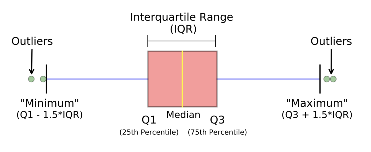
As we discussed previously, a boxplot shows the distribution of a numerical variable using five key values – the minimum, first quantile ($Q_1$), median, third quantile ($Q_3$), and maximum – and highlights any suspected outliers based on the interquartile range ($\text{IQR} = Q_3 - Q1$) rule.

7.2.3 Tukey’s IQR Rule

Tukey defined outliers as points that fall below $Q_1 - 1.5 * \text{IQR}$ or above $Q_3 + 1.5 * \text{IQR}$, providing a simple quantitative rule for detecting values that differ significantly from the main body of the data.

Tip

The coefficient $1.5$ is not fixed – it can be adjusted depending on the context and assumptions. However, in practice, the $1.5$ rule is the most commonly used standard.

We can define a function in R to find outliers based on the IQR rule:

Instead of creating a separate function, we can directly extract potential outliers using R’s built-in boxplot.stats()$out function, which applies Tukey’s IQR rule automatically.

As you can see, there are three potential outliers: two observations with a value of 44 and one with a value of 41.

We can easily find their row numbers in the dataset using the which() function.

With this information, you can now easily return to the corresponding rows in the dataset to verify them or review all variables for those observations.

Tip

This step helps verify whether these unusual observations are data entry errors or genuine extreme cases that may need special attention.

Tip

Another method to display these specific rows is with the identify_outliers() function from the {rstatix} package:

7.2.4 Standard deviation method

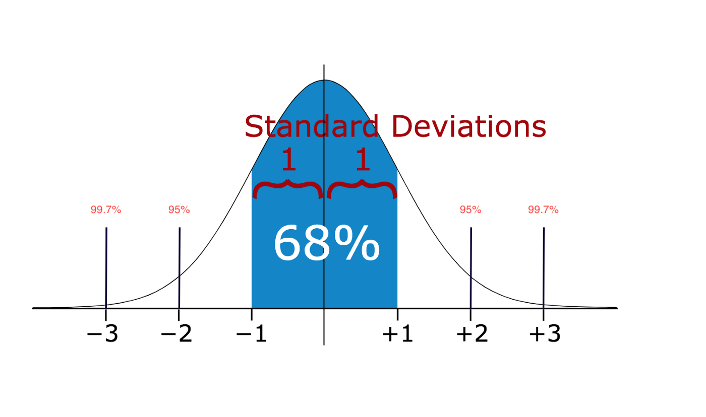
If the data follows a roughly normal (bell-shaped) distribution, we can use the standard deviation (SD) to identify outliers.

The standard deviation measures how far the data values are spread from the mean.

For a normal distribution:

$68\%$ of data lies within $\pm 1$ SD
$69\%$ of data lies within $\pm 2$ SD
$99.7\%$ of data lies within $\pm 3$ SD

Values that lie more than 2 or 3 SDs away from the mean are often considered potential outliers.

Note

This method can sometimes miss outliers because extreme values make the standard deviation larger.

7.2.5 $Z$-score method

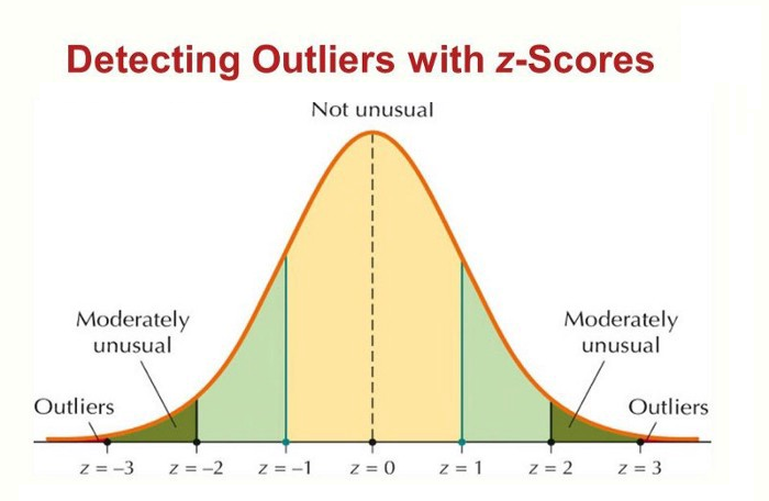
If the dataset follows a normal distribution, instead of the standard deviation method, we can transform the data into standard scores (or $Z$-scores) so that the mean becomes $0$ and the standard deviation becomes $1$.

This transformation gives us the $Z$-score for each observation, which indicates how many standard deviations an observation is from the mean. It can be done with the scale() function in R.

According to the empirical rule, observations with a $Z$-score greater than $3$ or less than $-3$ are considered as outliers (extremly rare). Values bewtween $|Z| = 2$ and $|Z| = 3$ are often described as “moderatly unusal” or rare.

Tip

Some analysts use a slightly stricter rule — considering values with $Z < −3.29$ or $Z > 3.29$ as outliers.

Why? The $Z = \pm 3$ rule comes from the empirical ($68$-$95$-$99.7$) rule, which is an approximately for normal distribution. It says that about $99.7\%$ of the data lies within $3$ standard deviations from the mean. That means roughly $0.3\%$ (or 3 in 1000) of observations would lie outside this range. However, if we calculate it more precisely from standard normal distribution, we find the $Z$-value that cuts off exactly $0.1\%$ in each tail (so that only %0.2%$ total or 2 in 1000 of obeservations lie beyond this point) is approximately $3.29$. So, $|Z| > 3$ means roughly $0.3\%$ of data, while $|Z| > 3.29$ means exactly $0.1\%$ per tail.

7.2.6 Modified $Z$-score method

The $Z$-score can be strongly affected by extreme values since it relies on the mean and standard deviation.

To make the method more robust, we use the modified $Z$-score, which is based on the median and median absolute deviation (MAD) instead.

The formula is: \[ \text{Modified $Z$-Score} = \frac{0.6745 (x_i - \text{Median})}{\text{MAD}} \] where $x_i$ is individual observation, and $\text{MAD}=\text{median}(|x_i - \text{median}(x_i)|)$.

Tip

The constant 0.6745 scales the MAD so that, under normality, the median absolute deviation estimates the standard deviation.

The MAD messures the spread of the data using the median instead of the mean, making it less sensitive to outliers than the standard deviation.

If the data are normally distributed, the standard deviation is typically preferref but for non-normal data, the MAD provides a more reliable measure of variablilty.

The outliers are identifed by \[ |\text{Modified $Z$-Score}| > 3.5 \] The value of $3.5$ was suggested by Iglewicz and Hoaglin (1993) in “How to Detect and Handle Outliers”, and is widely used because it balances sensitivity (detecting real anomalies) with robustness (avoiding false positives).

7.2.7 Hampel Filte

The Hample filter is an bust outlier detection method based on the median and the MAD – just like the modified $Z$-score method.

Instead of using the mean and standard deviation, it defines an interval around the median and flags as outliers any observations that fall outside this interval.

The interval is defined as: \[ I = [\text{Median} - k * \text{MAD}, \text{Median} + k * \text{MAD}] \] where $k$ is typically $3$.

This method is particularly useful for data that may not be normally distributed or when the dataset contains extreme values that could skew the mean and standard deviation.

7.2.8 Percentiles

The percentile method detects outliers by defining an interval that includes most of the data, based on selected percentiles. Any observations outside this interval are considered potential outliers.

The most common choice is to use the $2.5$th and $97.5$th percentiles, which corresponds to keeping $95\%$ of the central data and treating the remaining $5\%$ as potential outliers.

Other cutoff points, such as $1$st and $99$th or $5$th and $95$th percentiles, can also be used depending on how strict you want the detection to be.

7.3 What to Do After Detecting Outliers

Detecting outliers is only the first step — the most important part is deciding how to handle them. Outliers are not always “bad data” — they can be errors, rare but real events, or important signals.

The correct action depends on context and domain knowledge.

7.3.1 Verify and Investigate

Before taking any decision:

Check for data entry errors, unit mismatches, or measurement problems.
Plot the data again with and without outliers — see how much they influence the result.
Compare summaries (mean, median, variance) before and after removing outliers.

7.3.2 Keep the Outliers (if they are valid)

If the outliers represent real, meaningful phenomena, they should remain in the dataset. For example,

extremely high incomes in economics data
Rare but valid sensor readings in engineering.
Exceptional performance in experiments.

In such cases, you may use robust statistical methods (e.g. median, MAD) that are less sensitive to extreme values.

7.3.3 Remove or Winsorize (if they are incorrect)

If you find that the outliers come from a typographical or sensor errors, sampling issues, or wrong data units (e.g., °C vs. °F), then it’s reasonable to:

Remove them, or
Winsorize them — i.e., replace extreme values with the nearest valid percentile (e.g. 1st or 99th).

This keeps the data’s overall structure but limits the impact of extreme points.

7.3.4 Analyze With and Without Outliers

A good analytical habit is to perform the analysis both ways: once with all data and once excluding outliers. This helps assess how much the outliers influence the results and conclusions. If the results differ greatly, the outliers deserve closer attention.

7.3.5 Report Your Decision

Always document your reasoning:

Which method you used for detection,
How many outliers were found,
What you decided to do, and why.

Transparency ensures your analysis remains reproducible and credible.

7.4 Exercise

You are given the following dataset:

data <- c(
  47.19, 48.84, 57.79, 50.35, 50.64, 58.57, 52.30,
  43.67, 46.56, 47.77, 56.12, 51.79, 52.00, 50.55,
  47.22, 58.93, 52.48, 40.16, 53.50, 47.63, 44.66,
  48.91, 44.86, 46.35, 46.87, 41.56, 54.18, 50.76,
  44.30, 56.26, 52.13, 48.52, 54.47, 54.39, 54.10,
  53.44, 52.76, 49.69, 48.47, 48.09, 46.52, 48.96,
  43.67, 60.84, 56.03, 44.38, 47.98, 47.66, 53.89,
  49.58, 51.26, 49.85, 49.78, 56.84, 48.87, 57.58,
  42.25, 52.92, 50.61, 51.07, 51.89, 47.48, 48.33,
  44.90, 44.64, 51.51, 52.24, 50.26, 54.61, 60.25,
  47.54, 38.45, 55.02, 46.45, 46.55, 55.12, 48.57,
  43.89, 50.90, 49.30, 50.02, 51.92, 48.14, 53.22,
  48.89, 51.65, 55.48, 52.17, 48.37, 55.74, 54.96,
  52.74, 51.19, 46.86, 56.80, 46.99, 60.93, 57.66,
  48.82, 44.86, 100.58, 95.47, 81.32, 10.11, -1.87,
  -25.52, -34.14, -6.05, 20.78, 0.01
)

7.4.1 Part 1 — Using Tukey’s IQR Rule

Compute the first quartile (Q1), third quartile (Q3), and interquartile range (IQR).
Identify outliers using the standard $1.5 \times IQR$ rule.
Highlight them in a scatter plot.
How many potential outliers are there, and where are they located?

7.4.2 Part 2 — Using the Standard Deviation Method

Calculate the mean and standard deviation of the dataset.
Identify outliers as points that lie more than 2 standard deviations away from the mean.
Highlight them in a scatter plot.

7.4.3 Part 3 — Using the Z-score Method

Compute the Z-score for each observation (standardize the data).
Mark as outliers the values with $|Z| > 3$ (or $|Z| > 3.29$ for a stricter rule).
Compare your list of outliers with the ones found using the IQR method.
Plot both methods’ results — do they detect the same observations?

7.4.4 Part 4 – Discussion

Which method detected more outliers?
Are there points that one method flagged as outliers but not the other?
Which method do you think is more reliable for this dataset — and why?

7.4.5 Optional Challenge

Apply the Modified Z-score method or Percentile method (1%–99%) to the same dataset. Do the results change? What does that tell you about the robustness of different detection methods?