install.packages("dplyr")3 Data Wrangling
The dplyr package is a part of the R tidyverse : an ecosystem of several libraries designed to work together by representing data in common formats.
Caution
To load the dplyr package, you can install and load it as a standalone package or load the tidyverse.
Note
The data frame is a key data structure in statistics and in R. The basic structure of a data frame is that there is one observation per ro and each column represents a variable, a measure, feature, or characteristic of that observation. Given the importance of managing data frames, it is important that we have good tools for dealing with them.
The dplyr package is a relatively new R package that allows you to do all kinds of analyses quickly and easily.
Tip
It is especially useful for creating tables of summary statistics across specific groups of data.
One important contribution of the dplyr package is that it provides a “grammar” (in particular, verbs) for data manipulating and for operating on data frames. With this grammar, you can sensibly communicate what it is that you are doing to a data frame that other people can understand (assuming they also know the grammar). This is useful because it provides an abstraction for data manipulation that previously did not exist.
Important
Programming with dplyr look a lot different than programming in standard R. The dplyr works by combining objects (data frames and columns in data frames), functions (mean, median, etc.), and verbs (special commands in dplyr).
Important
In between the commands in dplyr is a new operator called the pipe which looks like this %>% or in the recent versions, like this |> . The pip tells R that you want to continue executing functions or verbs on the object you are working on. you can think about this pip as meaning ’and then …’
Note
Special commands called verbs because they “do something” to the data.
Some of the key “verbs” provided by the dplyr package are
select(): chooses certain columns, i.e., select variables by their names,filter(): extract certain rows, i.e, select observations by their values,mutate(): creates new variables/columns or transform existing variables,arrange(): reorders rows of a data framerename(): rename variables in a data framesummarise()/summarize(): gives summary information for different variables in data frame%>%or|>: the “pipe” operator is used to connect multiple verb actions together into a pipeline.
To install the dplyr package from CRAN, just run
Tip
Another way to get dplyr package is to install the whole tidyverse .
After installing the package, it is important to load it into the R session.
Warning
You may get some warnings when the package is loaded because there are functions in the dplyr package that have the same name ad functions in other packages.
Note
Note that all functions in the dplyr package require tidy data, which means that
each variable is in its own column,
each observation, or case, is in its own row
each value is in its own cell
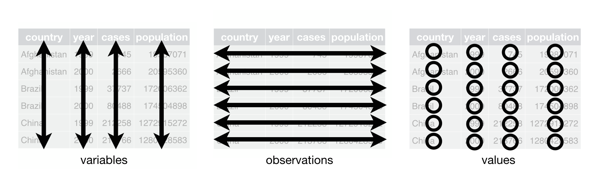
Rules of a tidy data frame: variables are columns, observations are rows, and values are cells. Source: @Wickham2023
To better understanding, let us continue within analyzing a dataset, penguins, available within the palmerpenguins package. we need to load the dataset and if it is necessary, we need to install the package.
# install.packages("palmerpenguins")

library("palmerpenguins")The data frame contain data for \(344\) penguins and \(8\) variables describing the species (species), the island (island), some measurements of the size of the bill (bill_length_mm and bill_depth_mm), flipper (flipper_length_mm) and body mass (body_mass_g), the sex (sex) and the study year (year). More information about the data frame can be found by running ?penguins .
You can see some basic characteristics of the dataset with the dim() and str() functions.
The first and last 6 rows can be displayed by head() and tail(), respectively.
The summary information of data frame can be found by summary() .
3.1 Filter observations - filter()
This function works on both quantitative and qualitative variables.
You can combine multiple conditions using & if all conditions must be true (cumulative), or | if at least one condition must be true (alternative). For example,
Note
Variable names should be used directly, without enclosing them in single or double quotation marks (' or ").
As you can see, the filter() functions require the name of the data frames as the first argument, then the condition (with the usual logical operators >, <, >=, <=, ==, !=, %in%, etc.) as second argument.
Caution
To use any functions in the dplyr package, you must specify the data frame’s name as the first argument. Alternatively, you can use the pipe operator (|> or %>% ) to avoid explicitly naming the data frame within each function.
Tip
The keyboard shortcut for the pipe operator is ctrl+shift+M on Windows or cmd + shift + M on Mac. By default, this will produce %>%, but if you have configured RStudio to use the native pipe operator, it will print |> .
Important
The pipe operator lets you chain multiple operations together, which is especially handy for performing several calculations on a data frame without saving the result of each intermediate step.
So with the pipe operator, the code above becomes:
Note
The pipe operator streamlines your code by feeding the output of one operation directly into the next, making your code much easier to write and read.
Instead of listing the data frame’s name as the initial argument within functions like filter() (or other {dplyr} functions), you simply specify the data frame once, then use the pipe operator to connect it to the desired function.
3.2 Extract observations
You can extract observations from a dataset based on either their positions or their values.
3.2.1 Based on Their Positions
To extract observations based on their positions, you can use the slice() function.
Furthermore, for extracting specific rows like the first or last, you can use specialized functions:
slice_head(): Extracts rows from the beginning of the dataset.slice_tail(): Extracts rows from the end of the dataset.
3.2.2 Based on their values
When you need to extract observations based on the values of a variable, you can use:
slice_min(): Selects rows with the lowest values, allowing you to define a specific proportion.slice_max(): Selects rows with the highest values, also with the option to define a proportion.
3.3 Sample Observations
Sampling observations can be achieved in two ways:
sample_n(): Takes a random sample of a specified number of rows.sample_frac(): Takes a random sample of a specified fraction of rows.
Note
It is important to note that, similar to the base R sample() function, the size argument can exceed the total number of rows in your data frame. If this happens, some rows will be duplicated, and you will need to explicitly set the argument replace = TRUE.
Alternatively, you can obtain a random sample (either a specific number or a fraction of rows) using slice_sample(). For this, you use:
The argument
nto select a specific number of rows.The argument
propto select a fraction of rows.
3.4 Sort observations
Observations can be sorted using the arrange() function.
By default, arrange() sorts in ascending order. To sort in descending order, simply use desc() within the arrange() function, like arrange(desc(variable_name)).
Similar to filter(), arrange() can sort by multiple variables and works with both quantitative (numerical) and qualitative (categorical) variables. For example, arrange(sex, body_mass) would first sort by sex (alphabetical order) and then by body_mass (ascending, from lowest to highest).
Important
It is important to note that if a qualitative variable is defined as an ordered factor, the sorting will follow its defined level order, not alphabetical order.
3.5 Select variables
You can select variables using the select() function based on their position or name.
To remove variables, use a - sign before their position or name.
You can also select a sequence of variables by name (e.g., select(df, var1:var5)).
Furthermore, select() provides a straightforward way to rearrange column order in your data frame.
3.5.1 Select using helper functions
The select() function also supports helper functions for matching column names based on patterns:
starts_with("abc") selects all columns whose names begin with the specified string.
ends_with("xyz") selects all columns whose names end with the specified string.
contains("ijk") selects all columns that contain the specified substring anywhere in their name.
The everything() helper selects all remaining columns that have not been explicitly mentioned. It is useful when you want to: move some variables to the front, or keep all others in their existing order.
num_range("prefix", 1:3) selects variables with names like "prefix1", "prefix2", "prefix3", etc. This is useful for selecting numbered variables.
matches("(.)\\1") selects columns whose names match a regular expression (regex).
This example selects aa and bb but not ab, since the pattern (.)\\1 means “a character repeated twice”.
3.6 Renaming Variables
To rename variables, use the rename() function.
Remember the syntax: new_name = old_name. This means you always write the desired new name first, followed by an equals sign, and then the current old name of the variable.
3.7 Create or Modify Variables
The mutate() function allows you to create new variables or modify existing ones. You can base these operations on another existing variable or a vector of your choice.
Note
If you create a variable with a name that already exists, the old variable will be overwritten.
Similar to rename(), mutate() requires the argument to be in the format name = expression, where name is the column being created or modified, and expression is the formula for its values.
There is another function transmute() that is also used to create a new variable in a data frame by transforming existing ones. However, unlike mutate(), which keeps all original columns and simply adds the new ones, transmute() returns only the newly created variables. This means that when you use transmute(), the resulting data frame will include just the variables you explicitly define inside the function. It is particularly useful when you want a clean output focused only on the transformed results, without retaining the original dataset’s columns. In contrast, mutate() is ideal when you want to preserve the full structure of your data while adding new insights.
Let us create a new column (body mass in kg).
3.8 Summarize Observations
To get descriptive statistics of your data, use the summarize() (or summarise()) function in conjunction with statistical functions like mean(), median(), min(), max(), sd(), var(), etc.
Remember to use na.rm = TRUE to exclude missing values from calculations.
3.9 Identify Distinct Values
The distinct() function helps you find unique values within a variable.
While typically used for qualitative or quantitative discrete variables, it works for any variable type and can identify unique combinations of values when multiple variables are specified. For instance, distinct(species, study_year) would return all unique combinations of species and study year.
3.10 Group By
The group_by() function changes how subsequent operations are performed. Instead of applying functions to the entire data frame, operations will be applied to each defined group of rows. This is particularly useful with summarize(), as it will produce statistics for each group rather than for all observations.
For example, to calculate the mean and standard deviation of body_mass separately for each species, you would first group_by(species) and then summarize() the body_mass. The pipe operator smoothly passes the grouped data from group_by() to summarize().
You can also group by multiple variables (e.g., group_by(var1, var2)), and the data frame’s name only needs to be specified in the very first operation of a chained sequence.
3.11 Managing Groups: ungroup()
After performing operations on grouped data, the ungroup() function allows you to revert to a normal data frame, enabling operations on entire columns again or switching to new grouping criteria. Remember, you can also group_by() multiple columns simultaneously.
3.12 Number of Observations
The function n() returns the number of observations. It can only be used inside summarize().
When combined with group_by(), you can easily get the number of observations per group. n() takes no parameters, so it’s always written as n().
Notably, the count() function is a convenient shortcut, equivalent to summarize(n = n()).
3.13 Number of Distinct Values
To count the number of unique values or levels in a variable (or combination of variables), use n_distinct(). Like n(), it’s exclusively used within summarize().
You do not have to explicitly name the output; the operation’s name will be used by default (e.g., summarize(n_distinct(variable))).
3.14 First, Last, or \(n\)th Value
Also available only within summarize(), you can retrieve the first, last, or nth value of a variable. Functions like first(), last(), and nth() enable this.
These functions offer arguments to handle missing values; for more details, consult their documentation (e.g., ?nth()).
3.15 Conditional Transformations
3.15.1 If Else
The if_else() function (used with mutate()) is ideal for creating a new variable with two levels based on a condition. It takes three arguments:
The condition (e.g.,
body_mass_g >= 4000).The output value if the condition is TRUE (e.g., “High”).
The output value if the condition is FALSE (e.g., “Low”).
Tip
A key advantage is that if_else() propagates missing values (NA) if the condition’s input is missing, preventing misclassification.
3.15.2 Case When
For categorizing a variable into more than two levels, case_when() is far more appropriate and readable than nested if_else() statements.
While nested if_else() functions can technically work, they are prone to errors and result in difficult-to-read code. For instance, to classify body mass into “Low” (<3500), “High” (>4750), and “Medium” (otherwise), nested if_else() would look like this:
This code first checks if body_mass_g is less than 3500. If true, it assigns “Low”. If false, it then checks if body_mass_g is greater than 4750. If that’s true, it assigns “High”; otherwise, it assigns “Medium”. While functional, this structure can become complex and error-prone with more conditions.
case_when() evaluates conditions sequentially. To improve this workflow, we now use the case when technique:
This workflow is much simpler to code and read!
If there are no missing values in the variable(s) used for the condition(s), it can even be simplified to:
While a .default argument can be used to specify an output for observations not matching any condition, exercise caution with missing values. If NA values in the conditioning variable are not explicitly handled, they might be incorrectly assigned to the default category. A safer approach is to explicitly define all categories or ensure NAs remain NA.
Note
Regardless of whether you use if_else() or case_when(), it’s always good practice to verify the newly created variable to ensure it aligns with your intended results.
3.16 Exploring Further dplyr Functions
Until now, we have focused on analyzing the penguins dataset. To effectively explain some of dplyr’s other powerful functions, we’ll now shift to creating custom datasets tailored to demonstrate their specific functionalities.
3.16.1 Separate and Unite
You can separate a character column into two or more new columns using separate().
Conversely, to combine two or more columns into a single character column, use unite().
3.16.2 Reshaping Data: gather() and spread()
gather() transforms “wide” format data into “long” or “tall” format by collapsing columns into key-value pairs.
Conversely, spread() converts “long” or “tall” format data into “wide” format by separating key-value pairs across multiple columns.
3.17 Combining Datasets: Joins
Sometimes, your data is split across multiple tables. For example, one table may have demographic information (like gender, marital status, height, weight), and another table may have medical records (like visits and surgeries).
When working with data spread across multiple tables, you’ll often need to combine them based on a shared column (a “key column”)—a process known as joining or merging. dplyr provides several functions for common data joins.
inner_join() keeps only the rows where “key column” exists in both tables and drops all rows that do not have a match in both.
lefy_join() keeps all rows from the left table (here, table1) and fills in matching information from the right table (here, table2). If no match is found, you will get NAs.
full_join() keeps all rows from both tables. Rows without a match in the other table will have NAs.
You can match on more than one column. For example, match ID and also make sure the gender in table1 matches sex in table2.
This is useful when one key (ID) is not unique enough by itself.
Filter-based joins: These do not add new columns. They just filter rows:
semi_join() keeps only rows in table1 that have a match in table2. It does not add any columns from table2.
anti_join() keeps only rows in table1 that do not have a match in table2. It is good for finding “missing” mathches.
Using the starwars dataset and dplyr functions, perform the following data manipulations.
Part 1: Initial Exploration and Filtering
Filter for Human Characters: Create a new data frame called
human_charactersthat only includes characters of the “Human” species.Select Key Attributes: From
human_characters, select only thename,height,mass, andhomeworldcolumns.
Part 2: Calculating BMI and Identifying Extremes
Calculate BMI: Add a new variable called
bmi(Body Mass Index) to yourhuman_charactersdata frame. The formula for BMI is \(\text{mass}/(\text{height}/100)^2\). Ensure thatmassis in kilograms andheightin centimeters as provided in the dataset.Sort by BMI: Arrange the
human_charactersdata frame in descending order based on theirbmi.
Part 3: Grouped Summaries
Species Statistics: Calculate the number of characters (
n) and the averageheightfor eachspeciesin the originalstarwarsdataset.Filter Significant Species: From the previous summary, filter out species that have fewer than 5 characters and an average height greater than 100.
Part 4: Conditional Categorization
Categorize Height: Add a new variable called
height_categoryto thestarwarsdataset usingmutate()andcase_when().If
heightis less than or equal to 100, categorize as “Short”.If
heightis greater than 100 but less than or equal to 180, categorize as “Medium”.If
heightis greater than 180, categorize as “Tall”.Handle
NAvalues forheightappropriately so they remainNAinheight_category.
Part 1: Initial Exploration and Filtering
Filter for Human Characters: which
dplyrfunction helps you select rows based on a condition? Remember the syntax for checking equality.There is a
dplyrfunction specifially for choosing columns.
Part 2: Calculating BMI and Identifying Extremes
Calculate BMI: Which
dplyrfunction is used to create or modify columns? Pay attention to the order of operations in the formula.Sort by BMI: The
arrange()function is key here. How do you specify descending order?
Part 3: Grouped Summaries
Species Statistics: You will need two main functions here: one to define groups and another to calculate summary statistics within those groups. Do not forget to handle
NAvalues for the mean.Filter Significant Species: You will apply another
filter()operation, but this time on the summarized data. Remember how to combine two conditions.
Part 4: Conditional Categorization
- Categorize Height:
case_when()is perfect for multiple conditions. How do you specify the conditions and their corresponding outputs? Remember to check forNAs first to ensure they do not get misclassified by other conditions.
Solution.
library(dplyr)

# Part 1: Initial Exploration and Filtering
human_characters <- starwars |>
  filter(species == "Human") |>
  select(name, height, mass, homeworld)

# Part 2: Calculating BMI and Identifying Extremes
human_characters_bmi <- human_characters  |>
  mutate(bmi = mass / ((height / 100)^2))  |>
  arrange(desc(bmi))

# Part 3: Grouped Summaries
species_stats <- starwars  |>
  group_by(species) %>%
  summarise(
    n = n(),
    avg_height = mean(height, na.rm = TRUE)
  ) %>%
  filter(
    n >= 5,
    avg_height > 100
  )

# Part 4: Conditional Categorization
starwars_with_height_category <- starwars %>%
  mutate(
    height_category = case_when(
      is.na(height) ~ NA_character_, # Handle NA values first
      height <= 100 ~ "Short",
      height > 100 & height <= 180 ~ "Medium",
      height > 180 ~ "Tall"
    )
  )
To learn more about the dplyr package, here are some recommended resources:
Chapter “Data transformation” in the book “R for Data Science”