Principal Component Analysis (PCA) is a technique used to replace a set of correlated variables by a smaller set of new, uncorrelated variables — the principal components — that retain as much of the original variability as possible.
Where clustering looks for structure among the rows of a data set (which clients resemble each other?), PCA looks for structure among the columns (which variables carry the same information?). The two questions are complementary, and in practice PCA is very often the step that comes before clustering or classification.
PCA was introduced by Pearson (1901) as a problem of fitting lines and planes to a cloud of points, and developed in its modern statistical form by Hotelling (1933). A comprehensive treatment is given by Jolliffe (2002).
10.1 Why Reduce Dimension?
A retail bank stores dozens — often hundreds — of numeric attributes per client: balances across several account types, transaction counts by channel, credit exposure, tenure, product holdings, contact history. An insurer stores a similar volume per policy. Working with all of them at once creates four practical difficulties.
Redundancy
Many variables measure the same underlying thing. A client’s income, current-account balance, savings balance, investment holdings and credit limit are all partial views of a single unobserved quantity we might call affluence. Keeping five columns to describe one construct adds noise, not information.
Multicollinearity
Strongly correlated predictors destabilise regression models: coefficients become large, sign-flipped and highly sensitive to small changes in the sample. Because principal components are uncorrelated by construction, they offer one way out of this problem.
Visualisation
We can look at a scatterplot of two variables, and with effort at a matrix of pairwise plots for five or six. We cannot look at a thirteen-dimensional cloud. PCA gives us the best possible two-dimensional “photograph” of that cloud, in a precise sense defined below.
The cost of dimension
Distances, densities and neighbourhoods behave badly in high dimension — the phenomenon usually called the curse of dimensionality. Since \(k\)-means, \(k\)-medoids and \(k\)-nearest-neighbours all rest on distances, reducing dimension first often improves both their speed and their results.
Note
PCA does not select a subset of the original variables. It builds new variables, each one a weighted combination of all the originals. If your goal is to discard columns and keep the rest (for example, because measuring each variable is expensive), PCA is the wrong tool — you want variable selection instead.
10.1.1 Applications in Banking and Insurance
Client segmentation
Reducing a wide client table to two or three interpretable axes — affluence, digital engagement, credit strain — and then clustering on those axes rather than on the raw variables.
Credit and behavioural scoring
Compressing correlated bureau and transaction variables into orthogonal components before fitting a scorecard, so that coefficient estimates remain stable.
Yield-curve and market-risk modelling
The classic financial application: applied to daily changes in interest rates across maturities, PCA almost always returns three components interpretable as level, slope and curvature, which together explain over 95% of yield-curve movement. Risk systems hedge these three factors instead of every maturity separately.
Insurance portfolio analysis
Summarising policyholder and claims characteristics (exposure, frequency, severity, coverage limits, bonus-malus level) into a small number of risk dimensions for tariff analysis or reinsurance decisions.
Fraud and anomaly detection
An observation that is poorly reconstructed from the first few components — that is, one lying far from the low-dimensional subspace where ordinary clients live — is a natural candidate for investigation.
Questionnaire and survey analysis
Identifying the latent dimensions behind a battery of customer-satisfaction items, which are typically far more numerous than the concepts they measure.
Packages and commands. No code in this section. The chapter uses stats for the analysis itself (prcomp, later varimax and promax), dplyr for the data preparation, factoextra and corrplot for the standard PCA figures, gridExtra to place figures side by side, and GPArotation for the rotation criteria that stats does not provide. All are installed and loaded by the setup chunk at the top of the chapter.
10.2 The Data: A Retail Bank Client Portfolio
Throughout this chapter we work with a simulated portfolio of \(600\) retail bank clients. The data are generated rather than downloaded so that every result in this chapter is exactly reproducible in your browser, but the variables, their units and their correlation structure are typical of a real retail banking table.
Variable
Type
Description
Unit
client_id
id
Anonymised client identifier
—
age
numeric
Age of the client
years
tenure
numeric
Time as a client of the bank
years
income
numeric
Declared annual net income
€
balance_current
numeric
Average balance, current account
€
balance_savings
numeric
Average balance, savings products
€
investments
numeric
Value of investment holdings
€
credit_limit
numeric
Total credit-card limit granted
€
utilization
numeric
Share of the credit limit in use
%
loan_balance
numeric
Outstanding loan and mortgage debt
€
card_tx
numeric
Card transactions per month
count
mobile_logins
numeric
Mobile-app logins per month
count
branch_visits
numeric
Branch visits per year
count
missed_payments
numeric
Missed payments in the last 24 months
count
segment
factor
Commercial segment: Mass / Affluent / Private
—
region
factor
Region of residence
—
churn
factor
Client closed the relationship in the last year
—
The code below creates the data set. Run it once: every interactive box in this chapter uses the object bank that it leaves behind.
Before any multivariate method, look at the marginal distributions. This is exactly the exploratory work of the EDA chapter, and it determines the choices we make next.
     income       balance_savings    investments      utilization
 Min.   :  4500   Min.   :    180   Min.   :    40   Min.   : 0.00
 1st Qu.: 18000   1st Qu.:   4368   1st Qu.:  1478   1st Qu.:19.10
 Median : 24950   Median :  10685   Median :  4930   Median :33.60
 Mean   : 30208   Mean   :  22762   Mean   : 17393   Mean   :34.41
 3rd Qu.: 37950   3rd Qu.:  24255   3rd Qu.: 13492   3rd Qu.:47.20
 Max.   :144500   Max.   :1209700   Max.   :577330   Max.   :99.00
 mobile_logins    missed_payments
 Min.   :  1.00   Min.   : 0.0000
 1st Qu.: 10.00   1st Qu.: 0.0000
 Median : 16.00   Median : 0.0000
 Mean   : 18.75   Mean   : 0.8717
 3rd Qu.: 24.00   3rd Qu.: 1.0000
 Max.   :184.00   Max.   :12.0000
10.2.1 Skewness and the Log Transform
The monetary variables are strongly right-skewed, as monetary variables almost always are: most clients hold modest amounts and a small number hold very large ones.
The savings balance has a skewness of \(15.1\) and investments of \(7.3\). PCA is a variance-based method, and variance is not robust: a handful of private-banking clients with balances two orders of magnitude above the median would, on the raw scale, define the first component almost by themselves. Taking logarithms of the monetary variables brings their skewness essentially to zero:
The same matrix is built in your browser session by the helper below. Every interactive box from here on begins with X <- make_X(), so you can run them in any order.
Tip
Log transformation of monetary variables before PCA is standard practice in banking and insurance analytics. It has three effects: it removes the dominance of a few very large clients, it turns multiplicative relationships (a client with twice the income tends to hold twice the savings) into additive ones, which is what linear methods can capture, and it makes the resulting components easier to read as differences in order of magnitude rather than in euros.
Beware of zeros: \(\log(0)\) is undefined. Common remedies are \(\log(x+1)\), or treating “holds no investments” as a separate binary variable.
The count variables card_tx, mobile and branch keep some skewness, which is normal for counts and not damaging at this level. We leave them untransformed so that their scale stays interpretable.
10.2.2 The Correlation Matrix
PCA is, in the end, a way of reading a correlation matrix. It is worth looking at that matrix directly first.
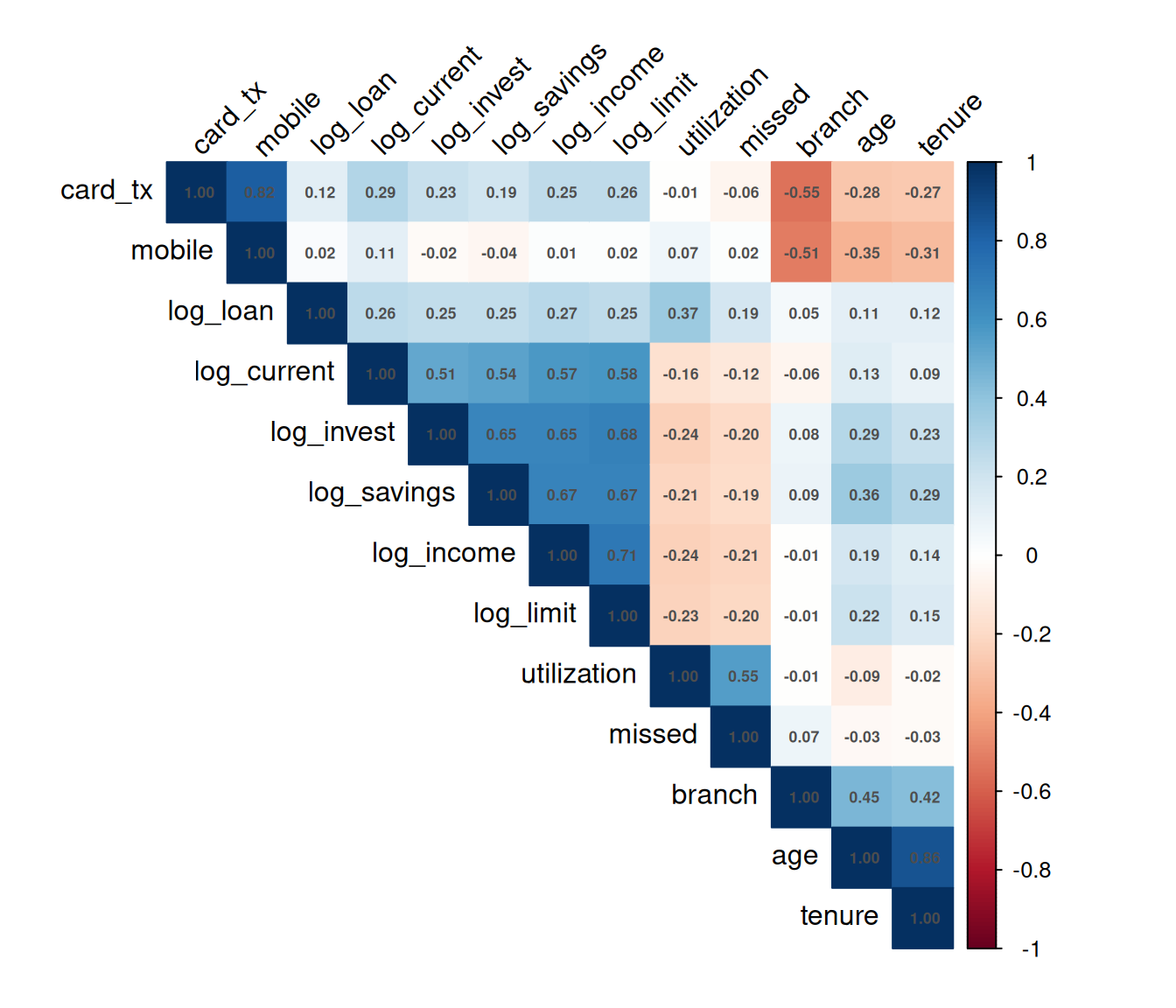
Correlation matrix of the transformed bank variables. Blocks of mutually correlated variables are exactly what PCA will summarise.
Three blocks stand out:
the monetary variables (log_income, log_savings, log_invest, log_limit, log_current) move together;
the channel variables (card_tx, mobile) move together and both move againstbranch, age and tenure;
utilization, log_loan and missed form a third, smaller block.
If the correlation matrix were the identity — all variables mutually uncorrelated — PCA would have nothing to do: every component would explain exactly \(1/p\) of the variance and no reduction would be possible. PCA is useful precisely to the extent that the variables are correlated.
Packages and commands. Simulation with set.seed, rnorm, rpois, runif and sample; marginal distributions with summary and sapply; the log transform with dplyr’s transmute; the correlation matrix with cor and corrplot’s corrplot(method = "color", order = "hclust"), whose order argument is what makes the blocks visible.
10.3 Pre-PCA Diagnostic Tests
The previous section ended on a qualitative statement: PCA is useful to the extent that the variables are correlated. Two classical diagnostics turn that statement into numbers, and they are routinely reported before a PCA:
Bartlett’s test of sphericity asks whether there is any correlation to summarise;
the Kaiser–Meyer–Olkin (KMO) measure asks whether that correlation is shared across many variables, which is what a small number of components can capture, or confined to isolated pairs.
Both come from the factor-analysis tradition. They do not decide whether PCA can be computed — it always can — but whether it is likely to produce a useful reduction.
10.3.1 Bartlett’s Test of Sphericity
Bartlett’s test (Bartlett 1950) tests the hypothesis that the population correlation matrix is the identity: \[
H_0: \mathbf{R} = \mathbf{I}_p
\qquad \text{versus} \qquad
H_1: \mathbf{R} \neq \mathbf{I}_p .
\] Under \(H_0\) the variables are uncorrelated and, in the language of the previous section, PCA has nothing to do. The test statistic is built from the determinant of the sample correlation matrix \(\hat{\mathbf{R}}\): \[
\chi^2 = -\left(n - 1 - \frac{2p + 5}{6}\right) \ln |\hat{\mathbf{R}}| ,
\] which, under \(H_0\) and multivariate normality, is approximately \(\chi^2\)-distributed with \(p(p-1)/2\) degrees of freedom.
The determinant is the natural quantity to look at. It equals the product of the eigenvalues of \(\hat{\mathbf{R}}\), so \(|\hat{\mathbf{R}}| = 1\) when the variables are uncorrelated and \(|\hat{\mathbf{R}}| \to 0\) as they become redundant — that is, as some eigenvalues approach zero. A small determinant means a large statistic.
bartlett_sphericity <-function(X) { R <-cor(X) n <-nrow(X) p <-ncol(X) stat <--(n -1- (2* p +5) /6) *log(det(R)) df <- p * (p -1) /2c(det =det(R), chisq = stat, df = df,p.value =pchisq(stat, df, lower.tail =FALSE))}signif(bartlett_sphericity(X), 4)
      det     chisq        df   p.value
6.974e-04 4.316e+03 7.800e+01 0.000e+00
The determinant is \(0.0007\), the statistic is \(\chi^2 = 4316\) on \(78\) degrees of freedom, and the \(p\)-value is zero to machine precision. The hypothesis of no correlation is rejected overwhelmingly.
That conclusion is less informative than it looks. The test has enormous power at realistic sample sizes, so it rejects for correlations far too weak to be worth summarising. Compare a matrix of pure noise of the same shape with the first \(30\) clients of our portfolio:
set.seed(1)noise <-matrix(rnorm(600*13), nrow =600, ncol =13)signif(bartlett_sphericity(noise), 4) # 600 x 13, no structure
    det   chisq      df p.value
 0.8788 76.7400 78.0000  0.5191
signif(bartlett_sphericity(X[1:30, ]), 4) # only 30 clients
      det     chisq        df   p.value
1.703e-05 2.617e+02 7.800e+01 1.090e-21
On noise the test correctly fails to reject (\(\chi^2 = 76.7\), \(p = 0.52\)); on just \(30\) clients it already rejects with \(p \approx 10^{-21}\). Passing Bartlett’s test is therefore a minimum requirement, not a recommendation: if it does not reject, stop — there is nothing for PCA to find. If it does, move on to KMO.
Warning
stats::bartlett.test() is not this test. It is Bartlett’s test for homogeneity of variances across groups, by the same author, and applying it to a data frame returns a meaningless result without an error. Use the function above or psych::cortest.bartlett().
The \(\chi^2\) approximation also assumes multivariate normality. Our count variables and the bounded utilization are clearly not normal, so treat the \(p\)-value as approximate — which, given how far it sits from any threshold, changes nothing here.
10.3.2 The Kaiser–Meyer–Olkin Measure of Sampling Adequacy
The KMO measure (Kaiser 1970, 1974) compares the ordinary correlations with the partial correlations — the correlation between two variables after the linear effect of all the others has been removed. The partial correlations are read off the inverse of the correlation matrix, \(\mathbf{Q} = \mathbf{R}^{-1}\): \[
a_{ij} = -\frac{q_{ij}}{\sqrt{q_{ii}\, q_{jj}}} .
\]
The logic is this. If variables \(i\) and \(j\) are correlated because both reflect a common underlying dimension that other variables also reflect, then controlling for those other variables removes most of the link and \(a_{ij}\) is small. If instead the two are linked only to each other, the partial correlation stays as large as the raw one. Components summarise the first kind of correlation, not the second.
The overall index compares the two sums of squares over all pairs \(i \neq j\): \[
\text{KMO} = \frac{\sum_{i}\sum_{j \neq i} r_{ij}^2}{\sum_{i}\sum_{j \neq i} r_{ij}^2 + \sum_{i}\sum_{j \neq i} a_{ij}^2} ,
\] and the measure of sampling adequacy of a single variable restricts the sums to its own column: \[
\text{MSA}_j = \frac{\sum_{i \neq j} r_{ij}^2}{\sum_{i \neq j} r_{ij}^2 + \sum_{i \neq j} a_{ij}^2} .
\] Both lie between \(0\) and \(1\). Values near \(1\) mean the partial correlations are negligible compared with the raw ones; a value of \(0.5\) is what uncorrelated noise produces. Kaiser’s own labels for the scale are still the ones in use:
KMO
Kaiser’s verdict
\(\geq 0.90\)
marvellous
\(0.80\) – \(0.89\)
meritorious
\(0.70\) – \(0.79\)
middling
\(0.60\) – \(0.69\)
mediocre
\(0.50\) – \(0.59\)
miserable
\(< 0.50\)
unacceptable
These labels are Kaiser’s verbal conventions from factor analysis, not inferential cut-offs: no sampling distribution stands behind them, and a middling value does not stop PCA from finding clear components, as the rest of this chapter shows.
The overall KMO is \(0.784\): middling, close to meritorious, and comfortably adequate for PCA. Pure noise gives \(0.491\), as expected.
The per-variable values are more instructive than the overall one. The five monetary variables all score between \(0.89\) and \(0.93\): their raw correlations with one another lie between \(0.51\) and \(0.71\), but their partial correlations only between \(0.06\) and \(0.31\), because the block explains each pair jointly. The lowest scores — utilization (\(0.61\)), mobile (\(0.64\)), tenure (\(0.66\)), card_tx (\(0.66\)), age (\(0.67\)) and missed (\(0.68\)) — belong to variables whose correlation is concentrated in one or two partners:
age and tenure are correlated at \(0.86\), and after removing the other eleven variables they are still correlated at \(0.81\): older clients have simply been clients for longer, and no other variable explains that. The same holds for card_tx and mobile (\(0.82 \to 0.79\)) and for the credit-strain trio. The monetary pair, by contrast, falls from \(0.65\) to \(0.20\): most of what links savings and investments is the affluence that every other monetary variable also measures.
A low MSA does not make a variable useless to PCA — these same variables will define the digital-engagement and credit-strain components later in the chapter. It says that their correlation is local, so that it takes a component to describe a small group of variables rather than a large one. The usual rule is to consider dropping variables with \(\text{MSA}_j < 0.5\), one at a time and starting from the lowest, recomputing after each removal. None of ours comes close, so all thirteen are kept.
ImportantWhen the diagnostics cannot be computed
KMO needs \(\mathbf{R}^{-1}\) and Bartlett needs \(\ln|\mathbf{R}|\), so both fail when \(\mathbf{R}\) is singular: when \(p \geq n\), or when one variable is an exact linear combination of others — a total alongside its parts, or a full set of dummy variables. solve then stops with an error and det returns zero. Remove the redundancy first. PCA itself still runs in these cases, and is often exactly the right tool for them; it is only the diagnostics that break.
Packages and commands. Both diagnostics need only base R: cor, det and pchisq for Bartlett’s statistic, and solve with the outer product %o% for the partial correlations behind KMO. The psych package wraps them as cortest.bartlett(R, n = ) and KMO(X). Do not confuse either with stats::bartlett.test, which tests equality of variances.
10.4 Notation, Centering and Scaling
Let \(\mathbf{X}\) be an \(n \times p\) data matrix: \(n\) clients in rows, \(p\) variables in columns. Write \(\mathbf{x}_i = (x_{i1}, \ldots, x_{ip})^{\top}\) for the record of client \(i\), and \(\bar{x}_j\) and \(s_j\) for the sample mean and standard deviation of variable \(j\).
10.4.1 Centering
PCA always begins by centering each variable: \[
\tilde{x}_{ij} = x_{ij} - \bar{x}_j .
\] Centering moves the origin of the coordinate system to the centre of gravity of the cloud of points. It is not optional: the components are directions through the mean, and without centering the first component would mostly point from the origin towards the mean of the data, which tells us nothing about its shape.
10.4.2 Scaling
Scaling is optional, and it is the single most consequential decision in a PCA. If we also divide by the standard deviation, \[
z_{ij} = \frac{x_{ij} - \bar{x}_j}{s_j},
\] then every variable has variance \(1\), and PCA is performed on the correlation matrix. If we do not, PCA is performed on the covariance matrix, and variables with large numerical variance dominate.
The variance of balance_savings is of the order of \(3.3 \times 10^{9}\) (euros squared); the variance of missed_payments is about \(2\) (counts squared). These numbers are not comparable — they are not even in the same units. A PCA on the covariance matrix of these columns is a PCA of the savings balance and nothing else:
The first component absorbs \(66.7\%\) of the variance and loads almost entirely on balance_savings and investments. Age, utilisation and every count variable have loadings indistinguishable from zero — not because they carry no information, but because they are measured in small numbers.
Warning
When variables are measured in different units, always use the correlation matrix (scale. = TRUE in prcomp, or cor = TRUE in princomp). Otherwise the analysis reflects your choice of units rather than the structure of the data: converting income from euros to thousands of euros removes it from the first component altogether (its loading falls from \(0.17\) to \(0\)), although nothing about the clients has changed.
The covariance matrix is appropriate only when all variables share the same unit and their differences in variability are themselves meaningful — for example, daily returns of a set of equities, or changes in yields across maturities.
From here on, every PCA is on the correlation matrix of the transformed matrix X.
Packages and commands.scale centres and standardises a matrix, and apply(X, 2, var) shows why that matters here. prcomp(X, scale. = TRUE) runs the PCA on the correlation matrix and scale. = FALSE on the covariance matrix; the older princomp makes the same choice through cor = TRUE.
10.5 The Algebra of PCA
10.5.1 The First Principal Component
Let \(\mathbf{Z}\) be the centred and scaled data matrix, and consider a direction in variable space given by a unit vector \(\mathbf{a} = (a_1, \ldots, a_p)^{\top}\), with \(\mathbf{a}^{\top}\mathbf{a} = 1\). Projecting the data onto this direction produces a new variable \[
y_i = \mathbf{a}^{\top}\mathbf{z}_i = a_1 z_{i1} + a_2 z_{i2} + \cdots + a_p z_{ip},
\qquad i = 1, \ldots, n ,
\] a linear combination of the original variables. Its sample variance is \[
\operatorname{Var}(y) = \mathbf{a}^{\top}\mathbf{S}\,\mathbf{a},
\] where \(\mathbf{S}\) is the sample covariance matrix of \(\mathbf{Z}\) — which, because the variables are standardised, is the correlation matrix\(\mathbf{R}\) of the original variables.
The first principal component is the direction that makes this variance as large as possible: \[
\mathbf{a}_1 = \arg\max_{\mathbf{a}^{\top}\mathbf{a} = 1} \; \mathbf{a}^{\top}\mathbf{S}\,\mathbf{a}.
\]
The constraint \(\mathbf{a}^{\top}\mathbf{a} = 1\) is essential: without it the variance could be made arbitrarily large simply by multiplying \(\mathbf{a}\) by a large constant, which changes the scale of the new variable but not the direction it points in.
Introducing a Lagrange multiplier \(\lambda\), we maximise \[
\mathbf{a}^{\top}\mathbf{S}\mathbf{a} - \lambda(\mathbf{a}^{\top}\mathbf{a} - 1),
\] and setting the derivative with respect to \(\mathbf{a}\) to zero gives \[
2\mathbf{S}\mathbf{a} - 2\lambda \mathbf{a} = \mathbf{0}
\qquad \Longleftrightarrow \qquad
\mathbf{S}\mathbf{a} = \lambda \mathbf{a}.
\]
This is the eigenvalue equation. The optimal direction \(\mathbf{a}\) must be an eigenvector of \(\mathbf{S}\), and its associated \(\lambda\) is an eigenvalue. Moreover, pre-multiplying by \(\mathbf{a}^{\top}\), \[
\mathbf{a}^{\top}\mathbf{S}\mathbf{a} = \lambda\, \mathbf{a}^{\top}\mathbf{a} = \lambda ,
\] so the variance captured by a component is its eigenvalue. To maximise variance we take the eigenvector belonging to the largest eigenvalue.
Note
Two readings of the same result:
Maximum variance: the first component is the direction along which the clients are most spread out.
Best fit: the first component is also the line that minimises the sum of squared perpendicular distances from the points to the line. This is the geometry of Pearson (1901), and it is not the same as the line fitted by ordinary least squares, which minimises vertical distances to a designated response variable.
Both descriptions define the same direction, which is why PCA can be presented either as variance maximisation or as low-dimensional approximation.
10.5.2 Subsequent Components
The second component solves the same problem with one extra requirement: it must be uncorrelated with the first. Since \[
\operatorname{Cov}(\mathbf{a}_1^{\top}\mathbf{z},\; \mathbf{a}_2^{\top}\mathbf{z}) = \mathbf{a}_1^{\top}\mathbf{S}\mathbf{a}_2 = \lambda_1 \mathbf{a}_1^{\top}\mathbf{a}_2,
\] requiring zero correlation is equivalent to requiring \(\mathbf{a}_1^{\top}\mathbf{a}_2 = 0\): the directions are orthogonal. Continuing in this way, the \(k\)-th component is the direction of maximum remaining variance among those orthogonal to the first \(k-1\).
Because \(\mathbf{S}\) is symmetric and positive semi-definite, it admits the spectral decomposition\[
\mathbf{S} = \mathbf{A}\,\boldsymbol{\Lambda}\,\mathbf{A}^{\top},
\qquad
\mathbf{A} = [\mathbf{a}_1, \ldots, \mathbf{a}_p],
\qquad
\boldsymbol{\Lambda} = \operatorname{diag}(\lambda_1, \ldots, \lambda_p),
\] with \(\lambda_1 \ge \lambda_2 \ge \cdots \ge \lambda_p \ge 0\) and \(\mathbf{A}^{\top}\mathbf{A} = \mathbf{I}\). The columns of \(\mathbf{A}\) are the \(p\) principal directions, sorted by the variance they explain, and they form an orthonormal basis: PCA is a rotation of the coordinate system, nothing more, until we decide to discard some of the new axes.
10.5.3 Total Variance is Preserved
Because the trace of a matrix is invariant under this rotation, \[
\sum_{k=1}^{p} \lambda_k = \operatorname{tr}(\mathbf{S}) = \sum_{j=1}^{p} s_{jj}.
\] On the correlation matrix every \(s_{jj} = 1\), so \[
\sum_{k=1}^{p} \lambda_k = p .
\]
With \(p = 13\) variables, the eigenvalues of our correlation matrix must sum to \(13\). This gives an immediate benchmark: a component with \(\lambda_k = 1\) explains exactly as much variance as one original standardised variable. This is the basis of the Kaiser criterion in Section 10.7.
The proportion of variance explained by component \(k\) is therefore \[
\text{PVE}_k = \frac{\lambda_k}{\sum_{m=1}^{p}\lambda_m} = \frac{\lambda_k}{p}
\quad \text{(correlation matrix)} .
\]
10.5.4 Connection with the Singular Value Decomposition
In practice, software does not form \(\mathbf{S}\) and diagonalise it; it applies the singular value decomposition to \(\mathbf{Z}\) directly: \[
\mathbf{Z} = \mathbf{U}\,\mathbf{D}\,\mathbf{V}^{\top},
\] with \(\mathbf{U}^{\top}\mathbf{U} = \mathbf{V}^{\top}\mathbf{V} = \mathbf{I}\) and \(\mathbf{D}\) diagonal with non-negative entries \(d_1 \ge \cdots \ge d_p\). Then \[
\mathbf{S} = \frac{1}{n-1}\mathbf{Z}^{\top}\mathbf{Z}
= \frac{1}{n-1}\mathbf{V}\mathbf{D}^{2}\mathbf{V}^{\top},
\] so \(\mathbf{V} = \mathbf{A}\) (the loadings) and \(\lambda_k = d_k^2/(n-1)\). The SVD route is numerically more stable, because squaring the data to form \(\mathbf{S}\) squares the condition number as well. This is why prcomp() (SVD-based) is preferred in R over the older princomp() (eigen-based).
Note
prcomp() divides by \(n-1\); princomp() divides by \(n\). The eigenvectors are identical, the eigenvalues differ by the factor \(n/(n-1)\), and for \(n = 600\) the difference is immaterial. Use prcomp().
10.5.5 Doing It by Hand
Everything above can be verified in a few lines. First the eigen-decomposition of the correlation matrix:
R_mat <-cor(X)e <-eigen(R_mat)round(e$values, 3) # the p eigenvalues
max(abs(abs(e$vectors[, 1]) -abs(pca$rotation[, 1]))) # first direction agrees
[1] 7.771561e-16
Both differences are of the order of \(10^{-14}\) — machine precision. And through the SVD:
Z <-scale(X) # centred and scaleds <-svd(Z)max(abs(s$d /sqrt(nrow(X) -1) - pca$sdev))
[1] 0
Identical again.
Warning
Signs are arbitrary. If \(\mathbf{a}\) is an eigenvector, so is \(-\mathbf{a}\), with the same eigenvalue. Different software — and different versions of the same software — may return a component with all its signs flipped. This changes nothing about the analysis, but it does reverse the verbal interpretation (“high on PC3” becomes “low on PC3”), so always state the direction explicitly when reporting results. This is why the comparison above uses abs().
10.5.6 A Two-Dimensional Picture of the Rotation
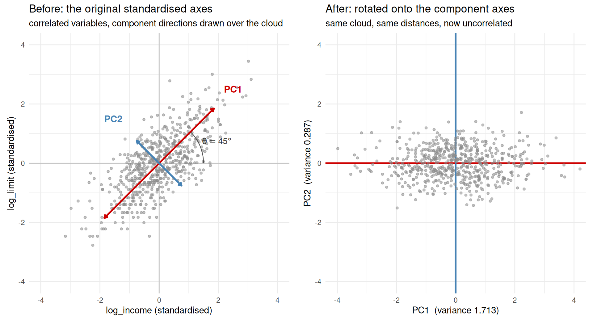
With thirteen variables the rotation cannot be drawn. With two it can, and the picture is worth more than the algebra. Take just log_income and log_limit — a client’s declared income and the card limit the bank granted them, which are related for an obvious reason.
pair <- X[, c("log_income", "log_limit")]pca2 <-prcomp(pair, scale. =TRUE)# both loadings come back negative; flip so that PC1 points up and to the rightpca2$rotation <--pca2$rotationpca2$x <--pca2$xcor(pair)[1, 2]
The correlation is \(r = 0.713\). The left panel below shows the two standardised variables with the component directions drawn over the cloud; the right panel shows the same clients after the rotation, plotted against their scores.
Left: two correlated standardised variables, with the component axes drawn over the cloud. Right: the same 600 clients plotted on those axes. Nothing has moved relative to anything else — the page has been turned by 45 degrees. Both panels use a 1:1 aspect ratio, without which a rotation does not look like one.
The elongated, tilted ellipse on the left becomes an ellipse aligned with the axes on the right. Three things are worth checking rather than believing:
# 1. distances between clients are unchanged: a rotation is a rigid motiond_before <-dist(scale(pair))d_after <-dist(pca2$x)max(abs(d_before - d_after))
[1] 1.776357e-15
# 2. total variance is unchanged, only redistributedc(before =sum(apply(scale(pair), 2, var)), after =sum(pca2$sdev^2))
before  after
     2      2
# 3. the new variables are uncorrelatedround(cor(pca2$x)[1, 2], 12)
[1] 0
The variables started with variance \(1\) each. After the rotation the same total of \(2\) is split \(1.713\) / \(0.287\) — that is, \(85.6\%\) of it now sits on a single axis. This is the whole of PCA in one line: the rotation does not create or destroy variance, it concentrates it.
Packages and commands.cor followed by eigen gives the eigenvalues ($values) and loadings ($vectors) by hand; svd gives the same through singular values ($d); prcomp does it in one call and is the one to use. dist checks that the rotation leaves every distance alone. The two-dimensional figure is ggplot2 plus gridExtra’s grid.arrange, and depends on coord_equal — without a 1:1 aspect ratio a rotation does not look like one.
10.6 Scores, Loadings and Explained Variance
Three objects come out of a PCA, and confusing them is the most common source of error in reading PCA output.
Object
Dimension
Meaning
In prcomp()
Loadings
\(p \times p\)
Weight of each variable in each component
$rotation
Scores
\(n \times p\)
Coordinate of each observation on each component
$x
Eigenvalues
\(p\)
Variance carried by each component
$sdev^2
10.6.1 Loadings
The loading \(a_{jk}\) is the weight of variable \(j\) in component \(k\). The vector \(\mathbf{a}_k\) has unit length, so the loadings of a component satisfy \(\sum_j a_{jk}^2 = 1\); a variable’s contribution to that component is therefore \(100\,a_{jk}^2\) per cent.
10.6.2 Scores
The score of client \(i\) on component \(k\) is \[
y_{ik} = \mathbf{a}_k^{\top}\mathbf{z}_i = \sum_{j=1}^{p} a_{jk}\, z_{ij}.
\] Scores are the new data: a client who was described by \(13\) numbers is now described by \(13\) new numbers, of which we intend to keep only the first few. By construction the scores have mean zero, variance \(\lambda_k\), and zero correlation with each other.
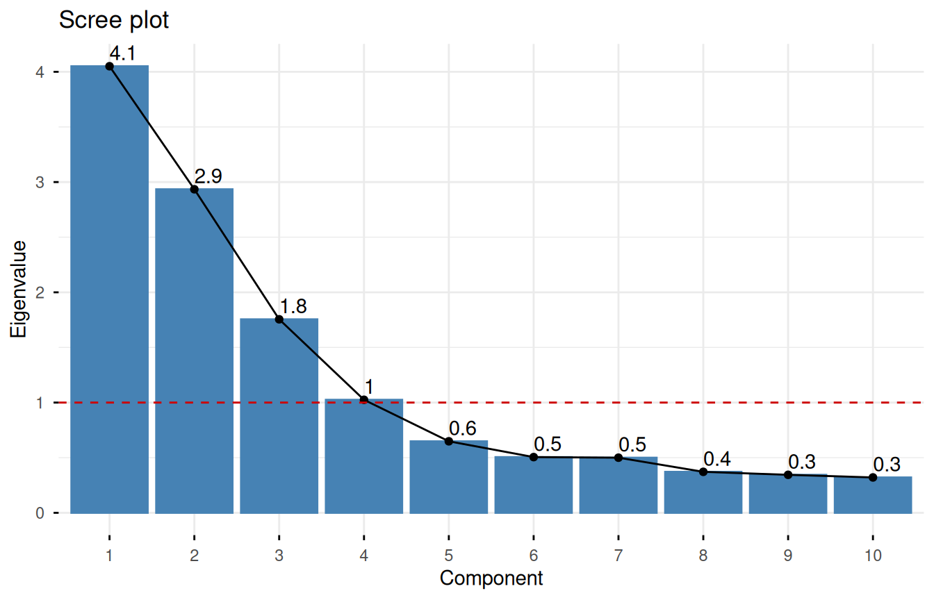
The eigenvalues are \(4.05\), \(2.93\), \(1.76\) and \(1.03\), explaining \(31.2\%\), \(22.6\%\), \(13.5\%\) and \(7.9\%\) of the total variance. The first three components together account for \(67.2\%\) of the variability of the thirteen original variables; adding the fourth brings this to \(75.1\%\).
Note
It is normal — and healthy — for social and behavioural data not to be compressible into two components. A first component explaining \(90\%\) of the variance usually means either that the variables are near-duplicates of one another, or that a scaling problem has gone unnoticed.
10.6.4 Reconstruction
Keeping only \(k\) components and rotating back gives an approximation to the standardised data: \[
\hat{\mathbf{Z}}_{(k)} = \mathbf{Y}_{(k)}\,\mathbf{A}_{(k)}^{\top},
\] where \(\mathbf{Y}_{(k)}\) holds the first \(k\) score columns and \(\mathbf{A}_{(k)}\) the first \(k\) loading columns. The Eckart–Young theorem (Eckart and Young 1936) states that this is the best possible rank-\(k\) approximation of \(\mathbf{Z}\) in the least-squares sense: no other set of \(k\) linear combinations reconstructs the data with smaller squared error.
Z <-scale(X)for (k inc(1, 2, 3, 4, 6, 8)) { Zhat <- pca$x[, 1:k, drop =FALSE] %*%t(pca$rotation[, 1:k, drop =FALSE])cat(sprintf("k = %d mean squared error = %.3f variance retained = %.1f%%\n", k, mean((Z - Zhat)^2), 100*sum(pca$sdev[1:k]^2) /ncol(X)))}
k = 1  mean squared error = 0.687   variance retained = 31.2%
k = 2  mean squared error = 0.462   variance retained = 53.7%
k = 3  mean squared error = 0.327   variance retained = 67.2%
k = 4  mean squared error = 0.248   variance retained = 75.1%
k = 6  mean squared error = 0.160   variance retained = 84.0%
k = 8  mean squared error = 0.093   variance retained = 90.7%
The error and the retained variance are two views of the same quantity: retaining \(67.2\%\) of the variance with three components means leaving \(32.8\%\) of it — a mean squared error of \(0.327\) on standardised data — in the discarded directions.
Packages and commands.prcomp returns $rotation (loadings), $x (scores) and $sdev (square roots of the eigenvalues). summary prints the variance table; factoextra’s get_eigenvalue returns the same thing as a data frame. Reconstruction is plain matrix algebra: pca$x[, 1:k] %*% t(pca$rotation[, 1:k]).
10.7 How Many Components to Retain?
There is no test that settles this question. The usual practice is to look at several criteria and take a decision that is defensible both statistically and substantively.
10.7.1 The Scree Plot
Plot the eigenvalues against their index and look for an “elbow” — the point after which the curve flattens into a scree slope of small, roughly equal eigenvalues (Cattell 1966). Components before the elbow are taken as signal, those after as noise.
Scree plot of the bank PCA. The curve bends after the third component; the fourth is borderline.
10.7.2 Cumulative Proportion
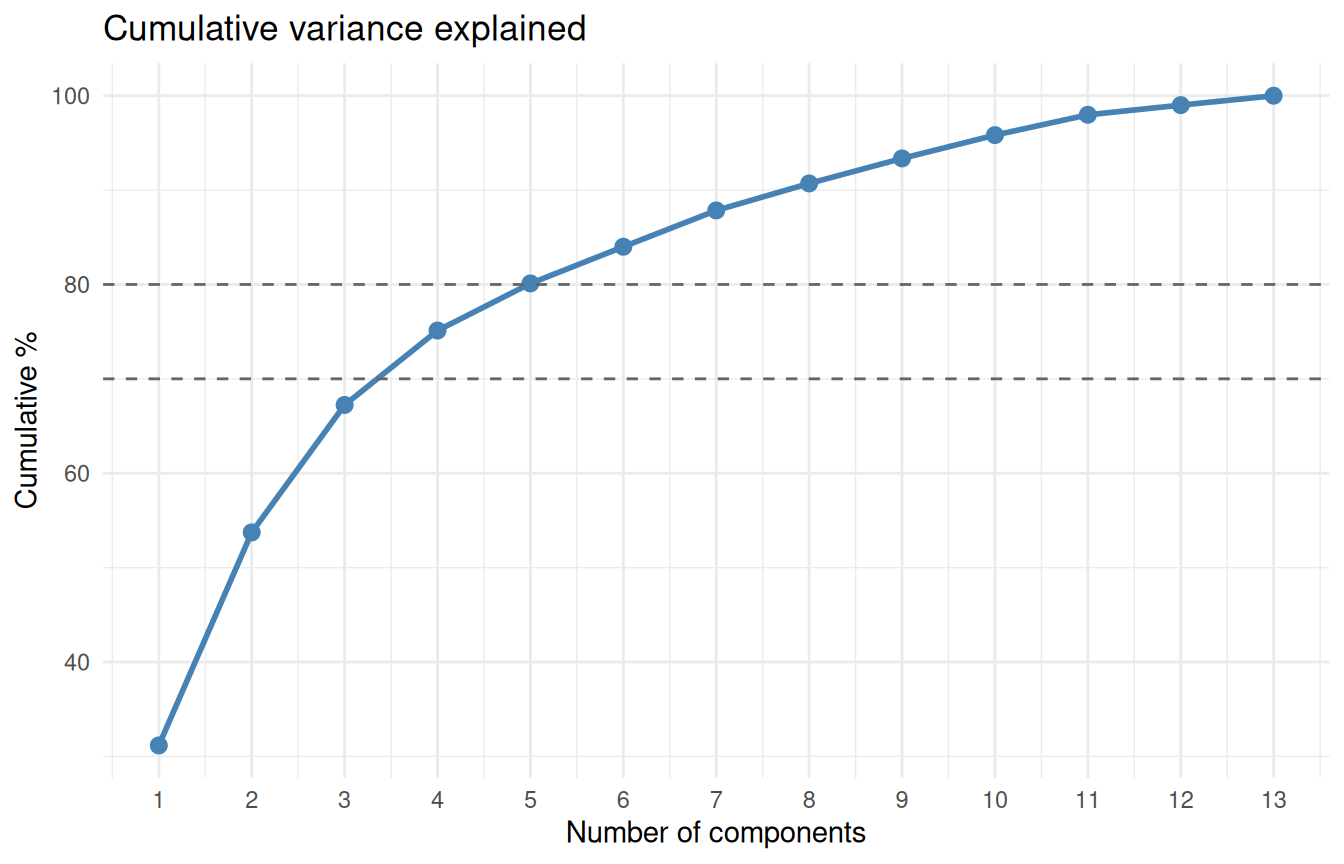
Retain as many components as needed to reach a target share of the total variance — commonly \(70\%\) or \(80\%\). The threshold is a convention, not a result, and should be chosen with the use in mind: a visualisation may be satisfied with two components, a preprocessing step for modelling usually wants more.
cum <-data.frame(comp =1:ncol(X), cum =cumsum(100* pca$sdev^2/ncol(X)))ggplot(cum, aes(comp, cum)) +geom_line(colour ="steelblue", linewidth =1) +geom_point(colour ="steelblue", size =2.5) +geom_hline(yintercept =c(70, 80), linetype ="dashed", colour ="grey40") +scale_x_continuous(breaks =1:ncol(X)) +labs(title ="Cumulative variance explained",x ="Number of components", y ="Cumulative %") +theme_minimal()
Cumulative percentage of variance explained. Three components pass 67%, four pass 75%.
10.7.3 The Kaiser Criterion
On the correlation matrix, retain components with \(\lambda_k > 1\)(Kaiser 1960). The logic is direct: a component explaining less than one standardised variable’s worth of variance is not a summary of anything.
Four components pass. Note how narrowly: \(\lambda_4 = 1.025\). A criterion that would drop a component if the fourth eigenvalue were \(0.99\) and keep it at \(1.01\) should not be applied mechanically.
10.7.4 The Broken-Stick Model
If a stick of unit length is broken at random into \(p\) pieces, the expected length of the \(k\)-th longest piece is \[
b_k = \frac{1}{p}\sum_{m=k}^{p} \frac{1}{m}.
\] Retain component \(k\) if it explains more variance than \(b_k\) — that is, more than would be expected if the total variance were divided among the \(p\) directions purely at random. This is a stricter rule than Kaiser’s, and generally a better-behaved one.
Broken-stick retains three components; Kaiser retains four. The disagreement is informative rather than annoying: it tells us the fourth component sits on the boundary between structure and noise, and we should decide it on interpretive grounds.
Tip
Summary of retention criteria
Criterion
Rule
Retains here
Comment
Scree / elbow
Bend in the eigenvalue curve
3
Visual, subjective, widely used
Cumulative %
Reach 70–80%
3–4
Threshold is a convention
Kaiser
\(\lambda_k > 1\)
4
Only for the correlation matrix; tends to over-retain
Broken stick
\(\lambda_k/p > b_k\)
3
Stricter, generally reliable
Interpretability
Can you name it?
3
The criterion that decides ties — but see Section 10.10
When criteria disagree, prefer the solution you can explain to the business. A component nobody can name is rarely worth carrying into the next stage of the analysis.
We retain three components for interpretation. Had the goal been prediction rather than explanation, keeping the fourth would have been defensible: a component that resists naming can still carry usable signal.
That is not quite the end of the question. Section 10.10 reopens it: a component that cannot be named as it stands may become nameable once the axes inside the retained subspace are rotated, and the fourth component of this portfolio is exactly such a case.
Packages and commands.factoextra’s fviz_eig(choice = "eigenvalue") draws the scree plot; cumsum and ggplot2 draw the cumulative curve. The Kaiser count is sum(pca$sdev^2 > 1), and the broken-stick values need no package at all — just sapply over the formula.
10.8 Visualising a PCA
10.8.1 The Variable Correlation Circle
Because the data are standardised, the correlation between variable \(j\) and component \(k\) is \[
r(x_j, y_k) = a_{jk}\sqrt{\lambda_k},
\] and these correlations are the coordinates used to plot variables on the correlation circle. Since a correlation cannot exceed \(1\) in absolute value, every variable lies inside a circle of radius \(1\).
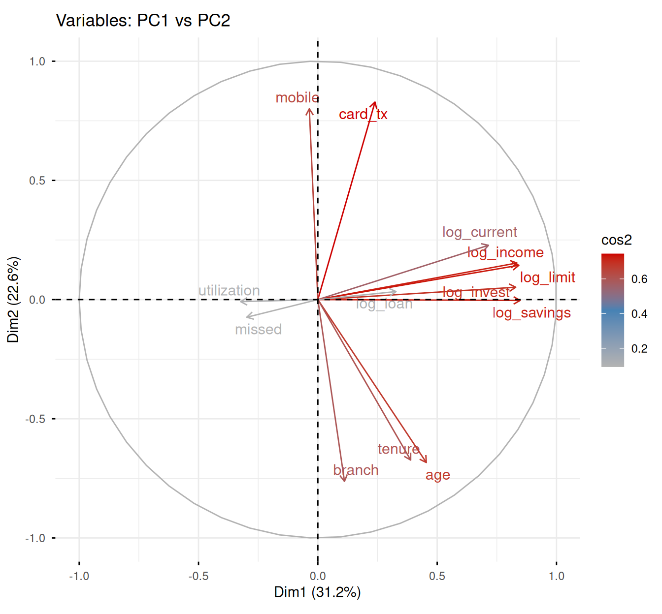
Variables on the plane of the first two components, coloured by quality of representation (cos2). Arrows close to the circle are well represented; small arrows are not.
How to read this plot:
Direction: variables pointing the same way are positively correlated; opposite directions mean negative correlation; a right angle between two well-represented arrows means near-zero correlation.
Length: the closer an arrow reaches the circle, the better the variable is represented by these two components. A short arrow means the variable lives mostly in other dimensions and should not be interpreted on this plane.
Position relative to the axes: an arrow lying along the horizontal axis defines PC1; one lying along the vertical axis defines PC2.
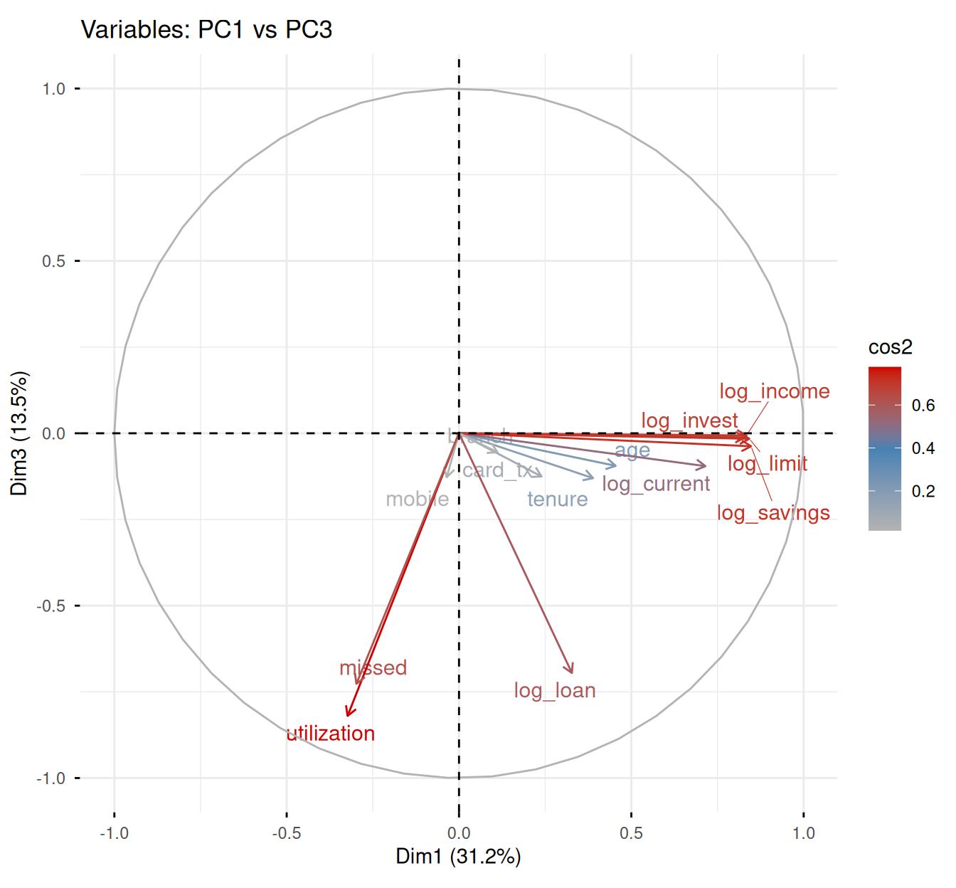
The monetary variables form a tight bundle along the positive horizontal axis. mobile and card_tx point up; branch, age and tenure point down. utilization, log_loan and missed have short arrows here — they belong to the third component, not to this plane.
Variables on the plane of components 1 and 3. The credit-strain block, invisible in the previous figure, appears clearly.
10.8.2 Quality of Representation: cos2
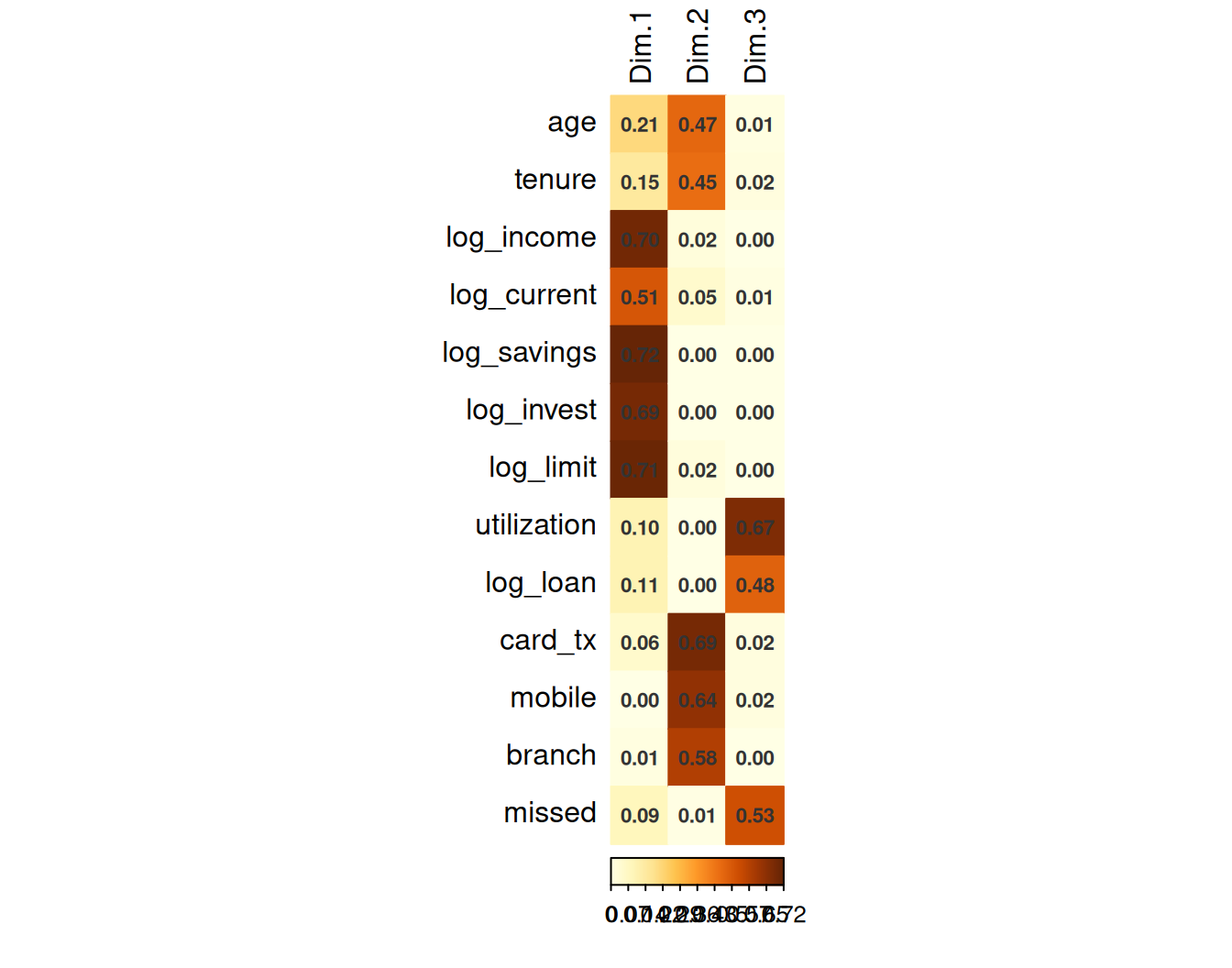
The quality with which variable \(j\) is represented by component \(k\) is the squared correlation \[
\cos^2(j, k) = r(x_j, y_k)^2 = a_{jk}^{2}\lambda_k ,
\] which is exactly the share of variable \(j\)’s variance recovered by component \(k\). Summing over all \(p\) components gives \(1\); summing over the retained ones gives the quality of representation on the chosen plane.
log_savings has \(\cos^2 = 0.718\) on PC1: nearly three quarters of its variability is captured by the first component alone. utilization has \(\cos^2 = 0.105\) on PC1 but \(0.672\) on PC3 — reading it on the first plane would be a mistake.
10.8.3 Communalities
The sum of the squared cosines of a variable over the retained components has a name of its own: it is the communality of that variable, \[
h_j^2 = \sum_{c=1}^{k} \cos^2(j, c) = \sum_{c=1}^{k} a_{jc}^{2}\lambda_c ,
\] where \(k\) is the number of components kept. It is the proportion of variable \(j\)’s variance that the retained components account for, and \(1 - h_j^2\) — the part they leave behind — is called the variable’s uniqueness or specific variance.
The name records what the quantity measures: the part of a variable that it holds in common with the others, in the sense that the retained components — which are built from all the variables at once — can reproduce it. What is left over, the uniqueness, is the part of the variable that the shared structure does not reach.
Two properties follow directly from the definition:
Over all\(p\) components the communality is exactly \(1\), since the components form a complete orthonormal basis. Communalities are only informative once some components have been discarded.
The average communality across the \(p\) variables equals the proportion of total variance retained. Communalities are therefore a decomposition, variable by variable, of the single global figure reported by the scree plot.
communality <-rowSums(var_info$cos2[, 1:3]) # three components retainedround(sort(communality), 3)
The two figures agree: \(0.672\), the \(67.2\%\) of total variance carried by the first three components.
Communalities are the natural check on whether a chosen number of components serves every variable or only most of them. Here they range from \(0.572\) for log_current to \(0.777\) for utilization — a narrow band, so no variable is being badly misrepresented by the three-component solution. A variable with a communality of, say, \(0.15\) would be a warning: it is nearly absent from the retained subspace, and any interpretation of the solution that mentions it would be unfounded. The usual responses are to retain another component, or to accept that the variable measures something the others do not share and to handle it separately.
Quality of representation of each variable on the first three components.
10.8.4 Contributions
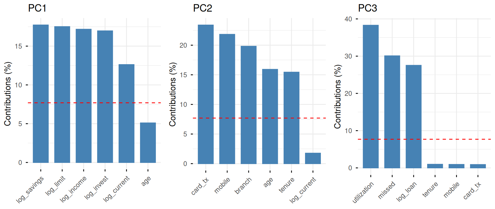
Where cos2 asks how well is this variable explained by the component, contribution asks the reverse: how much of this component is built from that variable. It is \[
\text{contrib}(j,k) = 100 \times a_{jk}^{2},
\] and the contributions of all variables to a given component sum to \(100\%\). The dashed reference line marks \(100/p\), the contribution a variable would have if all contributed equally.
library(gridExtra)g1 <-fviz_contrib(pca, choice ="var", axes =1, top =6, fill ="steelblue") +labs(title ="PC1")g2 <-fviz_contrib(pca, choice ="var", axes =2, top =6, fill ="steelblue") +labs(title ="PC2")g3 <-fviz_contrib(pca, choice ="var", axes =3, top =6, fill ="steelblue") +labs(title ="PC3")grid.arrange(g1, g2, g3, ncol =3)
Six largest contributions to each of the first three components. The dashed line is the contribution a variable would have under equal weighting (100/13 = 7.7%).
Note
Keep the two summaries apart. Contributions are read down a column — they say how much each variable builds a given component, and sum to \(100\%\) over the variables. Communalities are read along a row — they say how much of a given variable the retained components recover, and sum to \(1\) over all the components.
10.8.5 Individuals
The scores place each client on the new axes. Colouring them by a variable that did not take part in the PCA is one of the most useful checks available: if an external, meaningful grouping lines up with a component, the component is measuring something real.
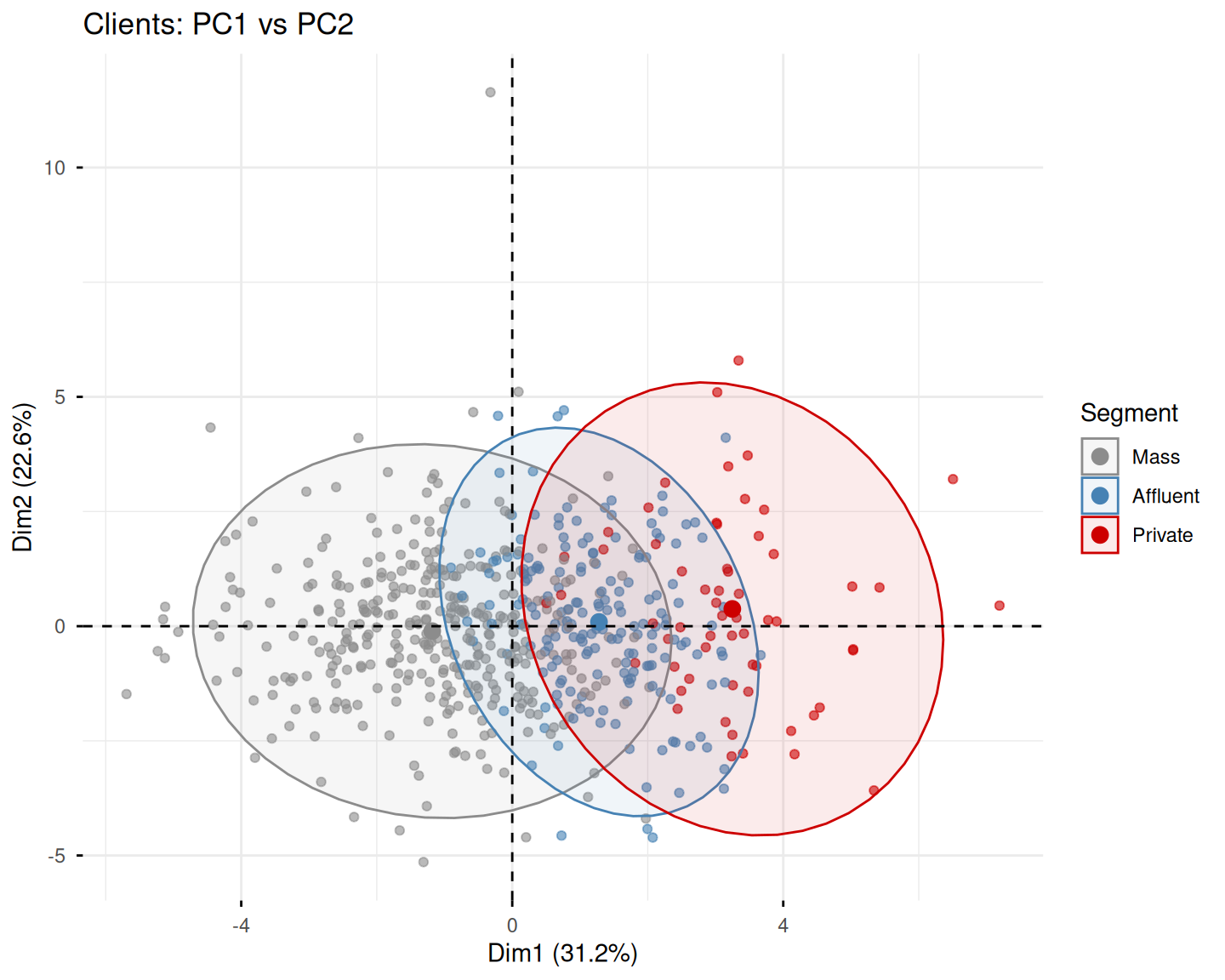
Mean PC1 rises from \(-1.18\) (Mass) through \(1.28\) (Affluent) to \(3.25\) (Private), while mean PC2 and PC3 barely move. This is strong external evidence that PC1 is an affluence axis.
10.8.6 The Biplot
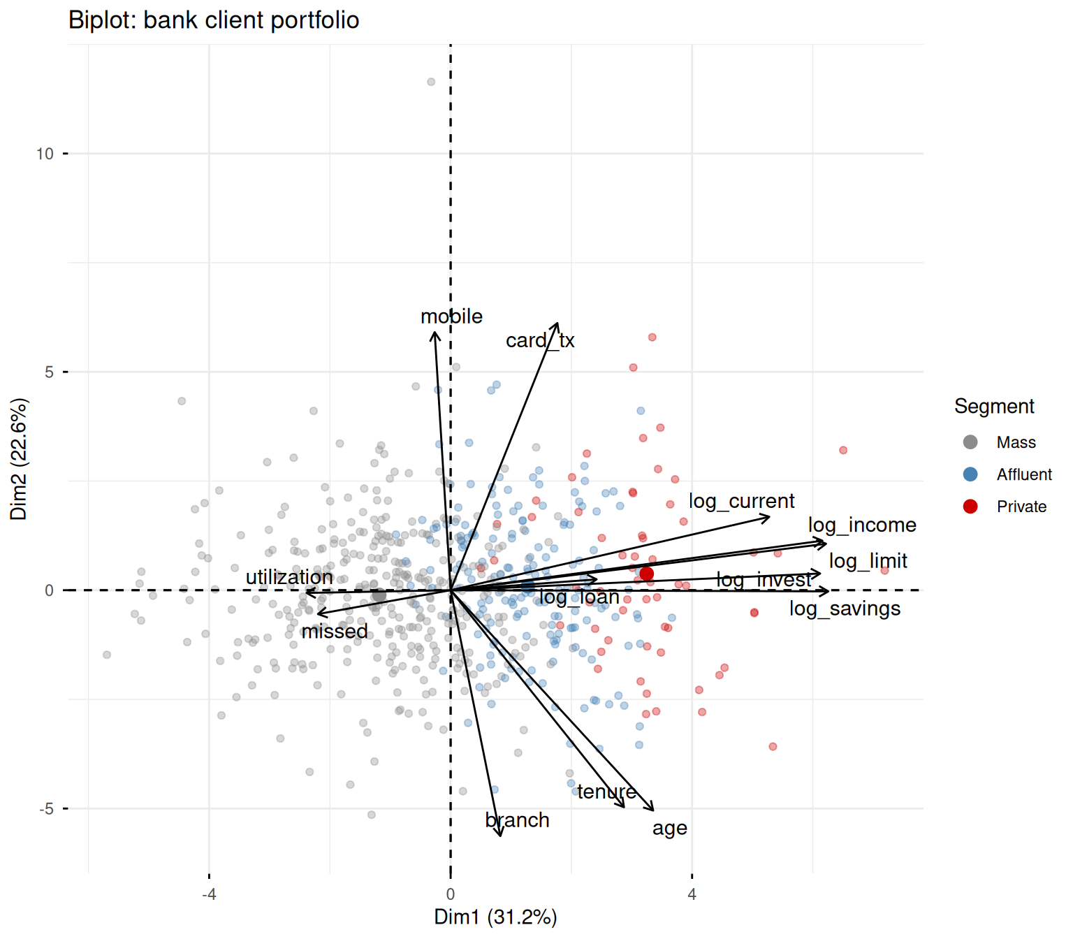
A biplot superimposes individuals and variables on the same plane. It is the most informative single figure of a PCA and also the easiest to over-read: the two sets of points are on different scales, and only their relative geometry is meaningful.
Biplot of the bank portfolio. Clients are positioned by their scores, variables by their loadings; a client lying far along an arrow has high values of that variable.
Note
Reading a biplot:
A client positioned in the direction of an arrow has an above-average value of that variable.
Clients far from the origin are atypical on the plane shown; clients near the origin are either average, or badly represented in these two dimensions. The two cases are distinguished by looking at the individual cos2, not at the plot.
The angle between two arrows approximates the correlation between the corresponding variables — but only when both arrows are long.
Packages and commands. All from factoextra: fviz_pca_var (correlation circle), fviz_contrib (contributions), fviz_pca_ind (individuals, with col.ind and addEllipses) and fviz_pca_biplot (biplot). get_pca_var returns the numbers behind those figures in $coord, $cos2 and $contrib. corrplot(is.corr = FALSE) displays a cos2 matrix, and aggregate summarises scores by an external grouping.
10.9 Interpreting the Components
A principal component has no meaning until someone gives it one. Interpretation proceeds by reading the loadings of a component and asking what the highly weighted variables have in common. Loadings below roughly \(0.3\) in absolute value are usually ignored as noise.
PC1 — Affluence (\(31.2\%\)). Large positive loadings on log_savings (\(0.421\)), log_limit (\(0.418\)), log_income (\(0.414\)), log_invest (\(0.412\)) and log_current (\(0.355\)); everything else is small. This is a size factor: a client high on PC1 has more of everything monetary. Its negative loadings on utilization (\(-0.161\)) and missed (\(-0.148\)) are weak but sensible — wealthier clients use less of their limit and miss fewer payments.
PC2 — Digital engagement versus branch and life stage (\(22.6\%\)). Positive on card_tx (\(0.484\)) and mobile (\(0.467\)); negative on branch (\(-0.445\)), age (\(-0.399\)) and tenure (\(-0.393\)). This is a contrast factor, and it says something the bank would care about: younger, shorter-tenure clients transact digitally, older and long-standing clients come to the branch. Note that PC2 is essentially uncorrelated with wealth — the digital divide in this portfolio runs along age, not income.
PC3 — Credit strain, reversed (\(13.5\%\)). Negative on utilization (\(-0.619\)), missed (\(-0.548\)) and log_loan (\(-0.525\)). A low score on PC3 means high utilisation, missed payments and large outstanding debt. Since it is easier to talk about a factor whose high values mean “more of the thing”, we can flip its sign:
After flipping, a high PC3 is a client under credit strain. The eigenvalue, the variance explained and every distance between clients are unchanged; only the label changes.
Warning
If you flip a component for readability, flip both the loadings and the scores, and do it once, at the start. Flipping only one of the two silently breaks the relationship \(\mathbf{Y} = \mathbf{Z}\mathbf{A}\) and every downstream result with it.
PC4 — a warning (\(7.9\%\)). The Kaiser criterion retained it (\(\lambda_4 = 1.025\)), but its loadings are a mixture: negative on tenure (\(-0.537\)), age (\(-0.479\)), mobile (\(-0.459\)) and card_tx (\(-0.371\)), with nothing else prominent. It appears to be a residual contrast between age and digital use after PC2 has taken the part of that contrast the two share. That is a statement about the geometry of the solution, not about clients. It is retainable for prediction and not interpretable as a construct — a distinction worth keeping.
Component
Variance
Name
High score means
PC1
31.2%
Affluence
High income, savings, investments and credit limit
PC2
22.6%
Digital engagement
Young, short tenure, transacts by card and app, rarely visits a branch
PC3 (flipped)
13.5%
Credit strain
High credit utilisation, missed payments, large debt
PC4
7.9%
—
No stable substantive reading
Tip
The interpretation above recovers, almost exactly, the four latent factors used to generate the data (W affluence, A life stage, D digital propensity, R credit risk) — although A and D were deliberately entangled and PCA, which is restricted to orthogonal directions, splits them across PC2 and PC4 rather than isolating each.
PCA recovers latent structure only up to a rotation. That is a real limitation, but it is also an opening: if the retained subspace is right and only the axes inside it are awkwardly placed, the axes can be turned. Section 10.10 does exactly that, and recovers all four factors — A included.
Packages and commands. No new tools: interpretation is reading pca$rotation, and flipping a component for readability is a minus sign applied to both $rotation[, k] and $x[, k].
10.10 Rotating the Components for Interpretation
Three of our four components had a clear reading; the fourth did not. That is a common outcome, and there is a standard response to it: keep the same set of retained components but turn the axes inside the subspace they span until the loadings fall into a pattern that is easier to name.
This is a different operation from the rotation of Section 10.5.1. There, rotating the axes was the PCA — the whole \(p\)-dimensional basis was turned so that the first axis caught the most variance. Here we take the \(k\) retained components as given and rotate only within them, deliberately giving up the maximum-variance ordering in exchange for readability.
10.10.1 Simple Structure
The target is what Thurstone (1947) called simple structure: a loadings matrix in which
each variable loads strongly on one component and near zero on the others,
each component has a handful of large loadings and many small ones,
few variables load on several components at once.
A matrix like that almost reads itself. The unrotated one rarely looks like that, because the first component is built to absorb as much variance as it can from every variable, which guarantees it has many moderate loadings.
Write \(\mathbf{L} = \mathbf{A}_k \boldsymbol{\Lambda}_k^{1/2}\) for the \(p \times k\) matrix of loadings on the retained components — the variable-component correlations of Section 10.8. A rotation replaces it by \[
\mathbf{L}^{*} = \mathbf{L}\,\mathbf{T},
\] with \(\mathbf{T}\) a \(k \times k\) orthogonal matrix chosen to make \(\mathbf{L}^{*}\) as close to simple structure as some criterion can measure. Throughout this section \(k\) is the number of retained components (the k of the code) and components are indexed by \(c\).
Warning
“Loadings” is used for two different matrices. Earlier in the chapter it meant pca$rotation, the eigenvectors, whose columns have unit length. Here it means \(\mathbf{A}_k\boldsymbol{\Lambda}_k^{1/2}\), whose entries are correlations and whose columns have squared sum \(\lambda_c\). Both are standard and both are called loadings; rotation is defined on the second, because simple structure is a statement about correlations. When you compare a printed table with pca$rotation, check which one you are holding.
Note
What a rotation preserves
the subspace spanned by the retained components, so the fitted values and the reconstruction error are unchanged;
every variable’s communality \(h_j^2\), and therefore the total variance retained.
What it gives up
the ordering: rotated components are no longer sorted by variance, and none of them is the maximum-variance direction any more;
the eigenvector property: they are no longer principal components, which is why they are conventionally written RC1, RC2, … rather than PC1, PC2, …;
uniqueness of the story: \(k\) must be chosen before rotating, and a different \(k\) gives a different rotated solution — not a nested one.
10.10.2 The Orthomax Family
Most orthogonal rotations maximise one criterion with one parameter changed: \[
Q(\mathbf{L}^{*}) \;=\; \sum_{c=1}^{k}\sum_{j=1}^{p} l_{jc}^{*4} \;-\; \frac{\gamma}{p}\sum_{c=1}^{k}\left(\sum_{j=1}^{p} l_{jc}^{*2}\right)^{2}.
\] Different \(\gamma\) give the named methods:
Method
\(\gamma\)
Simplifies
Behaviour
Quartimax
\(0\)
rows (variables)
Each variable loads on as few components as possible. Tends to leave one large general component.
Varimax
\(1\)
columns (components)
Each component gets a few large loadings. The default choice, and the one that most reliably produces nameable components.
Equamax
\(k/2\)
both
A compromise; spreads variance more evenly across components. Can be unstable.
Parsimax
\(p(k-1)/(p+k-2)\)
both
A further compromise, weighted by the problem’s dimensions.
Varimax (Kaiser 1958) is the one to reach for unless you have a reason not to.
GPArotation parameterises the same family through the Crawford-Ferguson constant \(\kappa = \gamma/p\), which is why equamax appears below as kappa = k / (2 * ncol(X)) rather than as \(\gamma = k/2\). The two are the same rotation.
10.10.3 Varimax on the Bank Portfolio
We rotate four components rather than three. The reason is the one Section 10.7 left unresolved: Kaiser retained four, broken-stick three, and we kept three because the fourth could not be named. Rotation changes that calculation, as we are about to see.
k <-4L <- pca$rotation[, 1:k] %*%diag(pca$sdev[1:k])dimnames(L) <-list(colnames(X), paste0("PC", 1:k))round(L, 3)
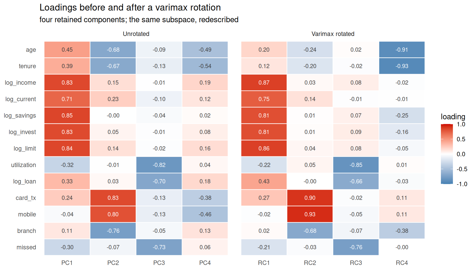
Loadings on four retained components, before and after a varimax rotation. The rotated panel is what simple structure looks like: one strong cell per row.
The rotated solution is far easier to read, and the change is not cosmetic:
RC1 — affluence. Unchanged in substance: income, savings, investments, limit, current balance, all above \(0.75\). Age has dropped out of it (\(0.45 \to 0.20\)).
RC2 — digital engagement. Now almost pure: card_tx\(0.90\), mobile\(0.93\), branch\(-0.68\). Age and tenure, which contributed \(-0.68\) and \(-0.67\) to the unrotated PC2, have fallen to \(-0.24\) and \(-0.20\).
RC3 — credit strain. Essentially untouched.
RC4 — life stage. The component that could not be named is now the cleanest of the four: age\(-0.91\), tenure\(-0.93\), and nothing else above \(0.4\). A high RC4 is a young, recently acquired client.
Rotation has separated the two constructs that the unrotated solution smeared across PC2 and PC4. Now check what it cost:
The total retained variance is \(75.1\%\) either way and no communality moves by more than \(10^{-15}\). What changed is the split: the first component gave up \(31.2\% \to 29.1\%\) and the second \(22.6\% \to 17.4\%\), while the fourth rose from \(7.9\%\) to \(15.0\%\) — and RC4 now explains more than RC3, so the components are genuinely no longer in order.
Tip
This is the honest argument for keeping the fourth component. Unrotated it was a \(7.9\%\) residual nobody could name; rotated it is a \(15.0\%\) life-stage factor with two loadings above \(0.9\). The number of components to retain and the decision to rotate are not independent questions.
The varimax row here is the unnormalised variant, so that all four solutions are scored on the same criterion; the rotation used above is the normalised default, which is why its first component carries \(29.1\%\) rather than \(28.5\%\).
Complexity is the average number of components a variable loads on: it falls from \(1.51\) unrotated to about \(1.21\) under any of the three rotations. On this portfolio the three orthogonal methods give practically the same answer — quartimax leaves slightly more variance on the first component, equamax slightly less, exactly as their definitions predict. When the three disagree materially, that is a sign the solution is not stable enough to name.
Warning
stats::varimax() applies Kaiser normalisation by default (normalize = TRUE): rows are scaled to unit length before rotating and rescaled afterwards, so that variables with small communalities still get a say. GPArotation does not normalise by default. The two therefore optimise slightly different things — on this data the raw criterion reaches \(0.3434\) without normalisation and \(0.3420\) with it. Neither is wrong, but a comparison across packages must hold the setting fixed.
10.10.5 Oblique Rotations
Orthogonal rotation keeps the components uncorrelated. That is a convenience, not a fact about the world: real constructs are often related, and forcing right angles can prevent simple structure from being reached at all. Oblique rotations — promax(Hendrickson and White 1964), oblimin, quartimin — drop the constraint.
Promax sharpens the loadings further — tenure reaches \(-0.997\) on RC4 and mobile\(0.984\) on RC2 — and it reports something an orthogonal rotation cannot: the components are correlated, and one pair substantially so. RC2 (digital) and RC4 (life stage) correlate at \(0.43\).
That number is not noise. The data were generated with D depending on A through the term \(-0.45\,\mathrm{A}\), which implies a correlation of about \(-0.49\) between digital propensity and life stage in the population, and \(-0.45\) in these 600 clients; RC4 loads negatively on age, making it a “youth” axis, which flips the sign. The oblique rotation has recovered a feature of the data-generating process that the orthogonal solutions, PCA and varimax alike, were constrained from showing.
Note
With an oblique rotation, read the pattern matrix (unique contribution of each component, printed above) for interpretation and the structure matrix (plain variable–component correlations, \(\mathbf{L}^{*}\boldsymbol{\Phi}\)) for a description of association. They differ precisely because the components overlap, and for the same reason the per-component variance shares no longer add up to the total — shared variance would be counted twice.
10.10.6 Rotated Scores
The scores rotate with the loadings, and they are what you carry into the next analysis. Since the matrix we rotated was \(\mathbf{L} = \mathbf{A}_k\boldsymbol{\Lambda}_k^{1/2}\) rather than the eigenvectors themselves, its partner is the standardised score matrix, and the rotation multiplies it on the right: \[
\mathbf{Y}^{*} = \mathbf{Z}\,\mathbf{A}_k\,\boldsymbol{\Lambda}_k^{-1/2},
\qquad
\mathbf{Y}^{*}_{\text{rot}} = \mathbf{Y}^{*}\mathbf{T}.
\] For an oblique rotation the same holds with \((\mathbf{T}^{\top})^{-1}\) in place of \(\mathbf{T}\), and the columns come out correlated — their correlation matrix is exactly \(\boldsymbol{\Phi}\).
Each column now reads as a score on a named construct: RC4 correlates \(-0.906\) with age, so it is a youth-and-recency index on a standard-deviation scale. The promax scores carry the \(0.43\) between digital engagement and life stage, so anything downstream that assumes uncorrelated inputs has to allow for it.
Warning
Two score conventions.prcomp()$x returns scores with variance \(\lambda_c\); the ones above have variance \(1\) in every column, because they are the partners of correlation-scaled loadings. Neither is wrong, but they are not interchangeable — \(k\)-means on the first weights the components by \(\lambda\), on the second equally. Say which you used.
10.10.7 When to Rotate, and When Not To
Caution
Rotate when the goal is to name and communicate constructs — a segmentation brief, a questionnaire’s underlying dimensions, a set of risk factors for a tariff discussion.
Do not rotate when the goal depends on the properties rotation destroys:
compression, where you want the fewest axes carrying the most variance;
a single index — a first component used as a wealth or vulnerability score — since after rotation no component is the best single summary;
any downstream use of the ordering, such as taking “the first two components”.
And whichever you do, say so. “The first four components explain 75%” and “the first four varimax-rotated components explain 75%, split 29/17/14/15 rather than 31/23/14/8” describe different objects.
Packages and commands.stats provides varimax (with normalize controlling Kaiser normalisation) and promax; both return $loadings and $rotmat. GPArotation supplies the rest of the family — quartimax, and cfT(kappa = ) for equamax — as well as the oblique oblimin and quartimin. The component correlation matrix is solve(t(rotmat) %*% rotmat), and rotated scores need solve and t as shown above.
10.11 Practical Issues
10.11.1 Outliers and Heavy Tails
PCA maximises variance, and variance is not a robust quantity. A single record far from the rest can rotate a component towards itself, producing a “component” that describes one client.
Suppose data-entry errors inflate the savings balance and the investment holdings of client C0001 to €50 million and €30 million; the true values are €22 020 and €77 560. We introduce the same error twice — once in the untransformed variables, once in the log-transformed ones — and compare.
On the log scale the corrupted record barely registers: the variance explained by the first three components moves from \(31.2\%\), \(22.6\%\), \(13.5\%\) to \(30.8\%\), \(22.6\%\), \(13.5\%\). On the untransformed scale the solution falls apart. Compare the first component before and after:
The correlation between the two versions of PC1 is \(-0.02\): the affluence factor has not been perturbed, it has been displaced entirely, and the first component of the corrupted analysis is now the age-versus-digital contrast. The affluence structure did not merely move down the ordering — the corrupted variables, having almost all their standardised variance concentrated in one point, are now nearly constant across the other \(599\) clients and no longer correlate with anything.
Where did the corrupted client go? Into a component of its own:
round(pca_rb$x[1, ] /apply(pca_rb$x, 2, sd), 1) # its scores, in standard deviations
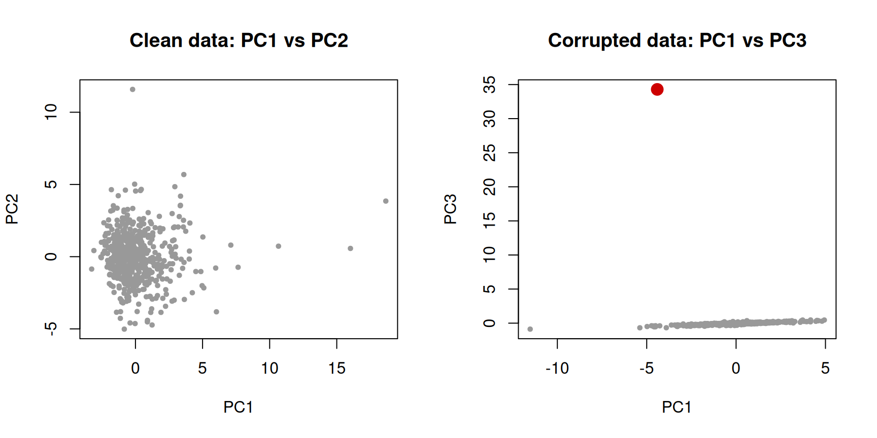
The third component of the corrupted analysis takes \(15.3\%\) of the total variance, loads \(0.70\) on each of the two corrupted variables and essentially zero on everything else, and the offending client sits \(24\) standard deviations along it. That component is not a description of the portfolio; it is a description of one typing mistake.
par(mfrow =c(1, 2))plot(pca_r$x[, 1], pca_r$x[, 2], pch =19, col ="grey60", cex =0.6,xlab ="PC1", ylab ="PC2", main ="Clean data: PC1 vs PC2")plot(pca_rb$x[, 1], pca_rb$x[, 3], pch =19, col ="grey60", cex =0.6,xlab ="PC1", ylab ="PC3", main ="Corrupted data: PC1 vs PC3")points(pca_rb$x[1, 1], pca_rb$x[1, 3], pch =19, col ="red3", cex =1.6)
Left: the clean untransformed analysis, where PC1 is affluence. Right: the same data with two corrupted cells, on the plane where the damage is visible. The third component of the corrupted analysis exists only to hold one client (red).
par(mfrow =c(1, 1))
All of this followed from an error in two cells of a table of \(7\,800\) values.
Tip
Notice what the log transform bought us. It did not remove the outlier — client C0001 still has an absurd balance — but it compressed errors of a factor of about \(2300\) (savings) and \(390\) (investments) on the euro scale to additive shifts of \(\log(2271) \approx 7.7\) and \(\log(387) \approx 6.0\) on the log scale, which are large but not catastrophic. Transformation is a cheap and effective first defence against exactly this failure mode. It is not a substitute for looking at the data.
Practical defences:
Screen for outliers before the PCA using the methods of the Outlier Detection chapter.
Distinguish errors from genuine extremes. A savings balance of €50 million is an error; a private-banking client with €1.2 million is a real client and should probably stay, possibly after a log transform.
Use the PCA itself as a diagnostic: an observation with a large score on a late, low-variance component, or a large reconstruction error, is atypical in a way the main structure does not explain.
Consider a robust PCA, based on a robust covariance estimator such as the MCD, when contamination is suspected and cannot be cleaned.
# reconstruction error per client using three componentsZhat <- pca$x[, 1:3] %*%t(pca$rotation[, 1:3])err <-rowSums((scale(X) - Zhat)^2)head(bank[order(err, decreasing =TRUE), c("client_id", "segment", "utilization","missed_payments", "mobile_logins")], 5)
    client_id  segment utilization missed_payments mobile_logins
272     C0272     Mass        76.5               3           184
308     C0308     Mass        86.3              12            17
231     C0231 Affluent         0.0               1             4
127     C0127     Mass        52.7               2             2
535     C0535     Mass        30.1               0            76
These are the clients least well described by the three-component summary — the natural shortlist for an anomaly review.
10.11.2 Missing Values
prcomp() has no mechanism for missing data: it removes any row with an NA, which can be a substantial part of the sample when many variables are involved. The options are those of the Missing Values chapter — deletion, single imputation, or multiple imputation — with one addition specific to PCA: iterative PCA imputation, which fills the missing cells with the values predicted by a low-rank reconstruction and iterates until convergence (implemented in the missMDA package).
Losing \(10\%\) of the sample to missingness in one variable is already noticeable; with missingness spread over several variables the loss compounds quickly.
10.11.3 Categorical Variables
PCA is defined for numeric variables. segment, region and churn cannot enter the analysis directly. Three options:
Leave them out and use them for illustration, as we did above — colouring the individuals plot by segment. This is the safest choice and often the most informative.
Dummy-code them. Workable for binary variables, but a dummy has variance \(\pi(1-\pi)\), which is small for rare categories; standardising then inflates rare categories and lets them drive components.
Use a method designed for the data type: Multiple Correspondence Analysis (MCA) for a set of categorical variables, or Factor Analysis of Mixed Data (FAMD) when numeric and categorical variables must be analysed together. Both are available in the FactoMineR package.
10.11.4 Multicollinearity and Near-Constant Variables
PCA tolerates perfect collinearity — the corresponding eigenvalue is simply zero — but a variable with zero variance breaks the standardisation, since dividing by \(s_j = 0\) is undefined. Check before scaling:
which(apply(X, 2, sd) ==0) # integer(0): no constant columns
named integer(0)
Also worth avoiding is including a variable twice in different guises (an amount and its logarithm, a total and its components). PCA will faithfully report that they are the same variable, and they will jointly dominate a component for no substantive reason.
10.11.5 Sample Size
PCA estimates \(p(p+1)/2\) covariances from \(n\) observations. With \(p = 13\) that is \(91\) quantities; \(n = 600\) is comfortable. Rules of thumb suggest at least \(5\)–\(10\) observations per variable, and more when the correlations are weak. With \(n < p\) the correlation matrix is singular and at most \(n-1\) eigenvalues are non-zero — PCA still runs, but the later components are pure artefact.
Packages and commands.na.omit shows the cost of listwise deletion, apply(X, 2, sd) finds constant columns, and the per-client reconstruction error is rowSums((scale(X) - Zhat)^2). Named but not used here: missMDA for iterative PCA imputation, FactoMineR for MCA and FAMD on categorical and mixed data, and a robust covariance estimator such as the MCD for robust PCA.
10.12 Common Pitfalls
Caution
Forgetting to scale when variables have different units — the analysis then reflects the units.
Interpreting a component before checking cos2 — a variable near the origin of the correlation circle is not “average”, it is absent from that plane.
Reading the sign of a component as meaningful — the sign is arbitrary; only the contrast is real.
Assuming the first component is the important one — it is only the largest. PCA orders components by variance in the variables, with no reference to any outcome you might later want to model, so importance depends on the question being asked.
Applying PCA to a set of uncorrelated variables — the eigenvalues will all be near \(1\) and nothing is gained. Look at the correlation matrix first.
Computing the PCA on the full data set before splitting into train and test sets — the test data then influence the transformation, and performance estimates are optimistic. Fit prcomp() on the training set and apply it with predict().
Treating principal components as causes — they are descriptive summaries of covariation, and nothing about the method licenses a causal reading.
Reporting components nobody can name without saying so — an uninterpretable component is a legitimate result, but it should be labelled as such.
# The correct way to use PCA inside a predictive workflowset.seed(42)idx <-sample(nrow(X), 0.7*nrow(X))pca_train <-prcomp(X[idx, ], scale. =TRUE) # fitted on training data onlyscores_tr <- pca_train$x[, 1:4]scores_te <-predict(pca_train, newdata = X[-idx, ])[, 1:4]
Packages and commands. The train/test pattern is the only code here: fit prcomp on the training rows, then apply the same transformation to the test rows with predict(pca_train, newdata = ). Never refit.
10.13 Beyond PCA: Other Routes to Fewer Dimensions
PCA makes three commitments: the new variables are linear combinations of the old ones, the criterion is global variance, and the whole \(n \times p\) matrix has to be decomposed at once. Each one is relaxed by a family of methods, and on large data the third becomes the binding constraint.
Multidimensional scaling (MDS) starts from a matrix of distances rather than from the variables themselves. Classical MDS — also called principal coordinates analysis — applied to Euclidean distances is not a rival to PCA; it is PCA:
mds <-cmdscale(dist(scale(X)), k =2)signif(max(abs(abs(mds) -abs(pca$x[, 1:2]))), 3) # identical, up to the sign of each axis
[1] 4.99e-14
The interesting case is the one PCA cannot reach. Feed MDS a dissimilarity that is not Euclidean — Gower’s coefficient for mixed numeric and categorical data, a correlation distance, an edit distance between strings — and you get a map of the clients even though no variable matrix exists. Non-metric MDS goes further still, preserving only the rank order of the dissimilarities, which is the right choice when the dissimilarities are ordinal.
Nonlinear methods drop the linearity. Kernel PCA runs an ordinary PCA in a feature space reached through a kernel. t-SNE and UMAP take a different view again: rather than preserving variance or global distance, they try to keep each point’s near neighbours near, which is what makes them so effective at showing clusters in high-dimensional data. UMAP is the faster of the two, keeps more of the global structure, and — unlike t-SNE — can place new points on an existing map.
On large data, the pressure is usually computational rather than conceptual, and it comes in two forms. With many rows and columns, a truncated or randomised SVD returns the leading \(k\) components without ever forming the full decomposition, and works on sparse matrices that would not fit in memory as a dense one. With very many columns, random projection is cheaper still: project onto random directions and, by the Johnson–Lindenstrauss lemma, pairwise distances survive to within a controllable error. Autoencoders — neural networks trained to reconstruct their own input through a narrow layer — are the nonlinear version of the same idea, and scale to data far beyond what prcomp will hold.
NIPALS — nonlinear iterative partial least squares(Wold 1966) — is the oldest algorithm that computes only the leading components. It never forms \(\mathbf{S}\). Each component is found by alternating two least-squares regressions on the residual matrix \(\mathbf{E}\), which starts as \(\mathbf{Z}\). Given a guess at the scores \(\mathbf{y}\), regress each column of \(\mathbf{E}\) on \(\mathbf{y}\) and normalise the coefficients to obtain the loadings \(\mathbf{a}\); then regress each row of \(\mathbf{E}\) on \(\mathbf{a}\) to update the scores, \(\mathbf{y} = \mathbf{E}\mathbf{a}\). Repeat until \(\mathbf{y}\) settles, then deflate, \(\mathbf{E} \leftarrow \mathbf{E} - \mathbf{y}\mathbf{a}^{\top}\), and start on the next component. Combining the two regressions gives \(\mathbf{a} \propto \mathbf{E}^{\top}\mathbf{E}\,\mathbf{a}\), so this is the power method, converging to the eigenvector of the largest remaining eigenvalue at a rate set by the ratio of the next eigenvalue to that one. Because each regression is a sum over cells, it can simply skip missing ones, and NIPALS gives a PCA of incomplete data without deleting any client — provided the cells are missing at random.
Method
Idea
In R
Classical MDS
Coordinates from a distance matrix; Euclidean case = PCA
cmdscale (stats)
Non-metric MDS
Preserve the rank order of dissimilarities
isoMDS (MASS), metaMDS (vegan), smacof
Kernel PCA
PCA in a feature space defined by a kernel
kpca (kernlab)
t-SNE
Preserve local neighbourhoods, for visualisation
Rtsne (Rtsne)
UMAP
As above, faster, and can map new points
umap (uwot)
Truncated / randomised SVD
The same leading components, computed cheaply
prcomp_irlba (irlba), RSpectra
NIPALS
Leading components one at a time by alternating regressions; tolerates missing cells
t-SNE and UMAP are for looking, not for measuring. They have no loadings, so no component can be named; they are stochastic, so two runs differ; and the distances between clusters, along with the apparent sizes of the clusters, carry no reliable meaning. Both depend strongly on a neighbourhood-size setting (perplexity, n_neighbors) that can manufacture groups that are not there.
For the kind of tabular client data in this chapter, PCA remains the default — it is deterministic, its components have loadings you can interpret, and predict applies the same transformation to new clients. Reach for a neighbour-embedding method when the goal is a picture of a high-dimensional space, and report it as a picture.
Packages and commands.cmdscale and dist are in stats; isoMDS is in MASS, which ships with R. Everything else is an install: vegan or smacof for non-metric MDS, kernlab for kpca, Rtsne and uwot for t-SNE and UMAP, irlba (prcomp_irlba) or RSpectra for truncated SVD on large or sparse matrices, nipals or ade4 (nipals) and the Bioconductor package pcaMethods for NIPALS, keras or torch for autoencoders.
10.14 Summary
PCA replaces \(p\) correlated variables by \(p\) uncorrelated components, ordered by the variance they explain, and is useful only to the extent that the original variables are correlated.
Check suitability before fitting. Bartlett’s test of sphericity must reject, but at realistic sample sizes it nearly always does; the KMO measure (\(0.78\) here) and the per-variable MSA say whether the correlation is shared widely enough for a few components to summarise it.
The components are the eigenvectors of the covariance (or correlation) matrix, and the variance each explains is the corresponding eigenvalue. Equivalently, they come from the SVD of the centred data matrix.
Centering is mandatory. Scaling is mandatory whenever the variables are in different units, which for client data is nearly always. Log-transform skewed monetary variables first.
The eigenvalues of a correlation matrix sum to \(p\), so a component with \(\lambda > 1\) explains more than one original variable.
Choose the number of components with several criteria at once — scree, cumulative variance, Kaiser, broken stick — and let interpretability settle the disagreements.
Loadings describe variables, scores describe observations, cos2 measures how well a variable is represented, contributions measure how much a variable builds a component, and the communality \(h_j^2\) — the sum of a variable’s squared cosines over the retained components — measures how much of that variable the reduced solution recovers.
In our bank portfolio, three components explaining \(67\%\) of the variance recover an affluence axis, a digital engagement versus branch axis, and a credit strain axis.
Rotating the retained components — varimax and its relatives — buys interpretability by giving up the variance ordering. It leaves the subspace, the communalities and the total retained variance untouched, and redistributes variance among the components. Here it turns an unnameable fourth component into the clearest factor of the four.
PCA is unsupervised: the largest component need not be the most useful for any particular downstream task.
10.15 Exercises
10.15.1 Exercise 1 — Scaling
Run a PCA on the raw (untransformed, unscaled) bank variables and compare it with the PCA on the correlation matrix of the transformed data.
What percentage of variance does the first component explain in each case?
Which variables have loadings above \(0.3\) on PC1 in each case?
Convert the six monetary variables (income, balance_current, balance_savings, investments, credit_limit, loan_balance) from euros to thousands of euros and re-run both analyses. Which one changes, and why?
10.15.2 Exercise 2 — Reproducing the output by hand
Using only cor(), eigen() and matrix multiplication:
Compute the eigenvalues of the correlation matrix of X and verify that they sum to \(13\).
Compute the scores of the first three components as \(\mathbf{Y} = \mathbf{Z}\mathbf{A}\), where \(\mathbf{Z}\) is the standardised data.
Verify that the score columns have variances equal to the eigenvalues, and that their pairwise correlations are zero.
Verify that \(\cos^2(j,k) = a_{jk}^2\lambda_k\) equals the squared correlation between variable \(j\) and score \(k\).
Hint: Y <- Z %*% e$vectors gives all the scores at once. Compare apply(Y, 2, var) with e$values, and round(cor(Y[, 1:3]), 10) with the identity matrix.
10.15.3 Exercise 3 — How many components?
For the PCA of X:
Produce the scree plot and state where you would place the elbow.
Apply the Kaiser criterion and the broken-stick model. They disagree — explain the disagreement in terms of \(\lambda_4\).
How many components are needed to reach \(80\%\) of the total variance? Is that a reasonable target here?
Examine the loadings of PC5 and PC6. Can you name either of them? Does that change your answer to (1)?
10.15.4 Exercise 4 — An insurance portfolio
Adapt the analysis to an insurance setting. The code below generates a portfolio of \(500\) motor policies.
Which variables should be log-transformed before the PCA? Justify with a skewness calculation.
claim_cost_3y is zero for policies with no claims. What does that do to a log transform, and how will you handle it?
Fit the PCA on the correlation matrix, decide how many components to keep, and name them.
Produce the correlation circle and the biplot, colouring policies by claims_3y > 0.
Compare your components with the two latent variables (V, B) used to generate the data. Did PCA recover them?
Rotate your retained components with varimax. Does the rotated solution separate the vehicle-and-coverage dimension from the driving-behaviour dimension more cleanly than the unrotated one? Compare each solution’s correlations with V and B.
10.15.5 Exercise 5 — Rotation and interpretation
Build the loadings matrix \(\mathbf{L}\) for three retained components and apply a varimax rotation. Compare it with the four-component rotation of Section 10.10. Does a clean life-stage factor appear? What does that tell you about the order in which “how many components?” and “rotate or not?” have to be decided?
Verify on your own solution that the rotation leaves every communality and the total retained variance unchanged, while changing the share carried by each component.
Return to the four-component solution of Section 10.10 (k <- 4) and rotate it with quartimax and with equamax as well. Which of the three leaves the most variance on the first component, and why is that exactly what its criterion is built to do?
On the same four components, run varimax() with normalize = TRUE and with normalize = FALSE. Report both criterion values and explain which variables Kaiser normalisation is protecting.
Apply promax() to the four-component solution. Report the component correlation matrix. Which pair of components is most strongly correlated, and does the code that generated bank account for it? Repeat with three components: what happens to that correlation, and why?
A colleague writes: “the first rotated component explains 29.1% of the variance, so it is the most important dimension in the portfolio.” Give two reasons to be careful with that sentence.
References
Bartlett, Maurice S. 1950. “Tests of Significance in Factor
Analysis.”British Journal of Statistical Psychology 3
(2): 77–85.
Bezdek, J. C., and R. J. Hathaway. 2002. “VAT: A Tool for Visual
Assessment of (Cluster) Tendency.”Proceedings of the 2002
International Joint Conference on Neural Networks. IJCNN’02 (Cat.
No.02CH37290) 3: 2225–30.
Brock, Guy, Vasyl Pihur, Susmita Datta, and Somnath Datta. 2008.
“clValid: An r Package for Cluster Validation.”Journal
of Statistical Software 25 (4): 1–22. https://doi.org/10.18637/jss.v025.i04.
Cattell, Raymond B. 1966. “The Scree Test for the Number of
Factors.”Multivariate Behavioral Research 1 (2):
245–76.
Charrad, Malika, Nadia Ghazzali, Véronique Boiteau, and Azam Niknafs.
2014. “NbClust: An r Package for Determining the Relevant Number
of Clusters in a Data Set.”Journal of Statistical
Software 61 (6): 1–36. https://doi.org/10.18637/jss.v061.i06.
Eckart, Carl, and Gale Young. 1936. “The Approximation of One
Matrix by Another of Lower Rank.”Psychometrika 1 (3):
211–18.
Gower, J. C. 1971. “A General Coefficient of Similarity and Some
of Its Properties.”Biometrics 27 (4): 857–71.
Hartigan, John A., and Manchek A. Wong. 1979. “A
K-Means Clustering Algorithm.”Applied
Statistics 28: 100–108.
Hendrickson, Alan E., and Paul O. White. 1964. “Promax: A Quick
Method for Rotation to Oblique Simple Structure.”British
Journal of Statistical Psychology 17 (1): 65–70.
Hotelling, Harold. 1933. “Analysis of a Complex of Statistical
Variables into Principal Components.”Journal of Educational
Psychology 24 (6): 417–41.
Jolliffe, Ian T. 2002. Principal Component Analysis. 2nd ed.
Springer.
Kaiser, Henry F. 1958. “The Varimax Criterion for Analytic
Rotation in Factor Analysis.”Psychometrika 23 (3):
187–200.
Kaiser, Henry F. 1960. “The Application of Electronic Computers to
Factor Analysis.”Educational and Psychological
Measurement 20 (1): 141–51.
Kaiser, Henry F. 1970. “A Second Generation Little Jiffy.”Psychometrika 35 (4): 401–15.
Kaiser, Henry F. 1974. “An Index of Factorial Simplicity.”Psychometrika 39 (1): 31–36.
Kaufman, Leonard, and Peter J. Rousseeuw. 1990. Finding Groups in
Data: An Introduction to Cluster Analysis. Wiley.
MacQueen, J. 1967. “Some Methods for Classification and Analysis
of Multivariate Observations.” In Proceedings of the Fifth
Berkeley Symposium on Mathematical Statistics and Probability,
edited by L. M. Le Cam and J. Neyman, vol. 1. University of California
Press.
Pearson, Karl. 1901. “On Lines and Planes of Closest Fit to
Systems of Points in Space.”The London, Edinburgh, and
Dublin Philosophical Magazine and Journal of Science 2 (11):
559–72.
Thurstone, Louis L. 1947. Multiple-Factor Analysis: A Development
and Expansion of the Vectors of Mind. University of Chicago Press.
Tibshirani, Robert, Guenther Walther, and Trevor Hastie. 2001.
“Estimating the Number of Data Clusters via the Gap
Statistic.”Journal of the Royal Statistical Society: Series
B (Statistical Methodology) 63 (2): 411–23.
Tukey, John Wilder. 1977. Exploratory Data Analysis.
Addison-Wesley Publishing Company.
Wickham, Hadley, Mine Cetinkaya-Rundel, and Garrett Grolemund. 2023.
R for Data Science: Import, Tidy, Transform, Visualize, and Model
Data. 2nd ed. https://r4ds.hadley.nz/.
Wickham, Hadley, Danielle Navarro, and Thomas Lin Pederson. 2019.
Ggplot2: Elegant Graphics for Data Analysis. 3rd ed. https://ggplot2-book.org/.
Wold, Herman. 1966. “Estimation of Principal Components and
Related Models by Iterative Least Squares.” In Multivariate
Analysis, edited by P. R. Krishnaiah. Academic Press.