13 Classification
Until now, we have been doing clustering – we had data with no labels, and we asked the computer to discover natural groups.
Now, we move to classification.
Suppose that we collected data from the engines on several ships: temperature, vibration level, and pressure. For each moment, we have numbers like \(\text{temperature} = 82^\circ \mathrm{C}\), \(\text{vibration} = 4.1\), and \(\text{pressure} = 205 kPa\).
At first, imagine we do not know if the engine was OK or about to fail at those moments. We just have the measurements. We ask the computer to group similar engine states together. The algorithm gives \(3\) groups:
- Group 1: normal temperature, low vibration
- Group 2: slightly higher temperature, medium vibration
- Group 3: very high temperature, very high vibration
Now, we look at Group 3 and we say that “This looks dangerous.”
It is very important that the algorithm never knew the words “safe” or “danger”. We discovered the groups and we interpreted them after. This is clustering.
Now, imagine we do have labels from the maintenance log. For every past moment, we know that
- Group 0 means the engine did not fail in the next 24 hours.
- Group 1 means the engine failed in the next 24 hours
We can train a model. The model sees examples like \((82^\circ \textrm{C}, 4.1 \textrm{vibration}, 205 \textrm{kPa})\) results in Group \(0\) (no failure) and \((96^\circ \textrm{C}, 7.5 \textrm{vibration}, 240 \textrm{kPa})\) results in Group \(1\) (failure). After training, we can give the model in the next 24 hours: yes or no? That task – taking a new case and predicting \(0\) or \(1\) – is called classification
There are several method that can act as classifiers, such as:
- logistic regression
- \(k\)-nearest neighbors
- decision trees and random forests
Here, we focus only on logistic regression.
13.1 Logistic regression
In many situation, we want to make a “yes/no” decision. For example:
- Is this email spam or not?
- Will this student pass or fail the exam?
- Is the fish a salmon or a sea bass?
- Is this transaction fraudulent or normal?
- will a loaner enter default or not, based on their credit score and income;
- will a driver be involved in an accident or not, based on their age, automobile age and driving history;
- will a patient have a heart attack or not, based on their cholesterol level and blood pressure, and other health indicators.
This kind of task is called a binary classification problem where the outcome variable can take on only two possible values. Usually we use \(0\) and \(1\) to denote two classes \(0\) and \(1\). For example, fail ( = \(0\)) vs. pass ( = \(1\)); normal (=\(1\)) vs. fault (=\(0\)), survived (=\(1\)) vs. died (=\(0\)).
Our goal is
Given information (variables) about something we have not seen before, can we decide if it is class \(0\) or class \(1\) based on what we learned from the previous labeled examples?
NoteDifference between clustering and Classification
In clustering, we did not know the groups in advance. We tried to discover “natural groups”.
In classification, we already know the correct group for past observations (they are labeled \(0\) or \(1\)). We used that labeled history to learn how to classify new observations in the future.
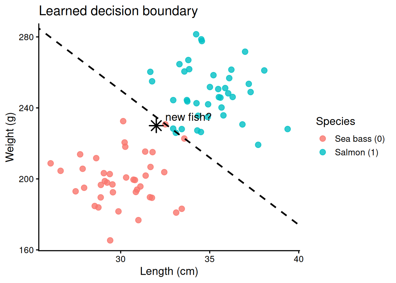
Imagine we are classifying fish using two measurements: length (cm) and weight (g).
Suppose we measured many fish, and for each fish we also know the species: \(1\) = salmon, and \(0\) = sea bass.
Now, we plot weight vs. length.
Based on the plot, we are seeing that each dot is a fish measured by length and weight; colors show the true species.
Now, imagine a new fish appears. We measure its length and weight. In the plot, the black star is a new fish. Where it lands on the plot will “look closer” to one group or the other.
Vary natural idea is > Let us just draw a line that separates salmon from sea bass.
The dashed line is the classifier’s decision boundary– the set of points where the model is 50-50 between the two classes.
So at this stage you can think:
- A classifier is something that finds a good decision boundary in the dataset.
- If a new point falls on one side, we say class 1. On the other side, it belongs to class 0.
This is already a valid mental model of classification.
Sometimes we do not want the answer.
We might see:
- Above or right of the line: the model predicts salmon (class 1)
- Below or left of the line: the model predicts see bass (class 0)
Because it sits below the boundary, the model predicts sea bass – but notice it is close to the line, so confidence is only moderate. Far from the line the model is more confident; near the line it is less sure.
The picture captures the core idea of classification: a model learns a good boundary from labeled data and uses it to decide the class of new points. Logistic regression is one such model that also gives a probability for class 1, with the boundary marking the 50% line.
So, at this stage, you can think:
- A classifier is something that finds a good decision boundary in your data.
- If a new point falls on one side, we can say class 1. On the other side, it belongs to class 0.
This is already a valid mental of classification. But we usually want more than just “yes/no”. We want to know how confident we are. For example, a medical model says a patient “has the disease”. That is important but not enough. We also want to answer some questions like “Is it \(99\%\) sure?” or “Is it \(52\%\) sure?” Those are very different situations in practice. This is where the logistic regression starts to shine:
- It does not just say “class 1” or “class 2”?
- It gives a probability that the observation is class 1.
For example,
- Probability this student will pass the exam is \(0.87\).
- Probability this transaction is fraus is \(0.12\).
- Probability this fish is salmon is \(0.71\)
Then, we, the human, or the company, or the doctor, can choose what to do.
This is a huge advantage: > Instead of a hard decision, we get a number between \(0\) and \(1\) that we can interpret as how likely it is to belong to class 1.
From a mathematical prespective, the problem statement can be like this.
We observed \(n\) labeled examples \[ \mathcal{D} = \{(\mathbf{x}_i, y_i)\}_{i=1}^n \qquad \mathbf{x}_i \in \mathbb{R}^p, \; y_i \in \{ 0, 1\} \] A classifier is a mapping \(h: \mathbb{R}^p \to \{ 0,1\}\) used to predict the label of a new feature vector \(\mathbf{x}\).
The ideal objective is to minimize \(0-1\) risk as \[ R(h) = Pr(h(X) \neq Y). \] Instead of optimizing the discontinuous \(0-1\) loss directly, we build a probablistic classifier \[ \pi_{\theta} (\mathbf{x}) = Pr(Y = 1 | \mathbf{X} = \mathbf{x}) \in (0,1) \] and then turn probabilities into decisions by a threshold \(\tau \in (0,1)\) as \[ \hat{y} (\mathbf{x}) = \begin{cases} 1, & \pi(\mathbf{x}) \geq \tau, \\ 0, & \text{otherwise} \end{cases} \] With the common choice \(\tau = 0.5\), the decision is “predict class 1 if it is more likely than class 0”.
Logistic regression specifies \(\pi (\mathbf{x})\) by applying the logistic (sigmoid) function to a linear score: \[ \pi_{\boldsymbol{\beta}}(\mathbf{x}) = \sigma(\eta) = \frac{1}{1 + e^{- \eta}}, \qquad \eta = \beta_0 + \mathbf{x}^{\top} \boldsymbol{\beta} \] or, equivalently, it assumes Bernulli conditional likelihood \[ Y | \mathbf{X} = \mathbf{x} \sim \text{Bernoulli}(\pi_{\boldsymbol{\beta}}(\mathbf{x})). \] Taking odds and log-odds gives the canonical logit link: \[ \text{logit}(\pi_{\boldsymbol{\beta}}(\mathbf{x})) = \log \left( \frac{\pi_{\boldsymbol{\beta}}(\mathbf{x})}{1 - \pi_{\boldsymbol{\beta}}(\mathbf{x})} \right) = \beta_0 + \mathbf{x}^{\top} \boldsymbol{\beta} \]
Geometry For a threshold \(\tau\), the decision boundary is the hyperplane \[ \beta_0 + \mathbf{x}^{\top} \boldsymbol{\beta} = \text{logit}(\tau). \] With \(\tau = 0.5\), this reduces to \(\beta_0 + \mathbf{x}^{\top} \boldsymbol{\beta} = 0\) (a straight line in 2D, a plane in 3D).
Interpretation A one-unit increase in variable \(x_j\) (holding others fixed) changes the log-odds by \(\beta_j\) and multiplies the odds by \(e^{\beta_j}\) (an odds ratio).
Estimation by Maximum Likelihood Given the dataset \(\mathbf{D}\), the log-likelihood under the Bernoulli model is \[ \ell(\boldsymbol{\beta}) = \sum\limits_{i=1}^n [y_i \log(\pi_i) + (1 - y_i) \log(1 - \pi_i)], \qquad \pi_i = \sigma(\beta_0 + \mathbf{x}^{\top}\boldsymbol{\beta}). \] The maximum likelihood estimator (MLE) of \(\hat{\boldsymbol{\beta}}\) maximizes \(\ell(\boldsymbol{\beta})\), or equivalently minimizes the negative log-likelihood (binary cross-entropy): \[ \mathcal{L}(\boldsymbol{\beta}) = - \ell(\boldsymbol{\beta}) = \sum\limits_{i = 1}^n [- y_i \log(\pi_i) - (1 - y_i) \log(1 - \pi_i)] \]
A binary classification problem is one where the outcome variable can take on only two possible values. For example:
- will a loaner enter default or not, based on their credit score and income;
- will a driver be involved in an accident or not, based on their age, automobile age and driving history;
- will a patient have a heart attack or not, based on their cholesterol level and blood pressure, and other health indicators.
For this kind of problem, the dataset used to fit the model is composed of observations \((\mathbf{x}_1, y_1)\), \((\mathbf{x}_2, y_2)\), …, \((\mathbf{x}_n, y_n)\) where each \(y_i\) is usually labelled 0 (failure, no event, …) or 1 (success, event, …) and \(\mathbf{x}_i\) is a vector of input variables.
The task at hand is to build a model that, given an arbitrary \(\mathbf{x}\), will predict the probability that \(y = 1\).
13.2 Modelling Probabilities
Why not use a linear regression model to predict the probability that \(y = 1\)? After all, linear regression is a well-known and widely used method.
There are some problems with this approach:
- the output values are never (with probability 1) exactly 0 or 1, the values that are taken by \(y\);
- even considering a threshold (e.g. 0.5) to classify the predicted values into 0 or 1, this would be mostly an arbitrary chosen value.
13.3 Sigmoid Functions
Instead of a linear function, we can opt to model the probability of success of the event described by \(y\), i.e \(\operatorname{P}(Y=1)\). This is a more sound and natural way to model the prediction of a random binary event. In order to do this, we can use sigmoid functions. A sigmoid function \(f(x)\) is a function having an “S” shaped curve (sigmoid curve) with the following properties:
- \(0<f(x)<1\);
- \(\displaystyle \lim_{x \to -\infty} f(x) = 0\), \(\displaystyle \lim_{x \to +\infty} f(x) = 1\);
- \(f'(x)>0\).
A common sigmoid function is the logistic function, defined as:
\[ f(x) = \frac{e^x}{1 + e^x} = \frac{1}{1 + e^{-x}}. \]
A logistic function can be used to model the probability that \(y = 1\) given \(\mathbf{x}\).
This function will play a central row in the logistic regression model, as we will see briefly.
13.4 Logistic Model
The first random variable that comes to mind in order to model a random binary event is the Bernoulli random variable, which is a discrete random variable that takes value 1 with probability \(p\) and value 0 with probability \(1-p\). The parameter \(p\) is the probability of success of the event described by the random variable, and it’s probability function is
\[ p(y) = p^y (1-p)^{1-y}, \quad y \in \{0, 1\}. \] The expected value of a Bernoulli random variable is \(\operatorname{E}[Y] = p\) and it’s variance is \(\operatorname{V}(Y) = p(1-p)\).
Note
A natural extension is the Binomial random variable, which is the sum of \(n\) independent Bernoulli random variables with the same parameter \(p\). The parameter \(p\) is again the probability of success of the event described by the random variable, and it’s probability function is
\[ p(y) = \binom{n}{y} p^y (1-p)^{n-y}, \quad y \in \{0, 1, ..., n\}. \]
Another way of expressing the probability of an event is through the odds of the event, defined as the ratio between the probability of the event and the probability of it’s complementary event:
\[ \operatorname{odds} = \frac{p}{1-p} = \frac{1}{1-p^{-1}}, \quad p \in ]0, 1[. \]
The odds are a number between 0 and \(+\infty\). If the odds are equal to 1, then the event and it’s complementary are equally likely. If the odds are greater than 1, then the event is more likely than it’s complementary event, and vice versa. It’s easy to see that odds are monotonically increasing with respect to \(p\):
\[ {(\operatorname{odds})}' = \frac{1}{(1-p)^2} > 0. \]
Odds are an alternative way of expressing probabilities, still being relatively intuitive concerning interpretation. Nevertheless, they are still confined to the interval \(]0, +\infty[\), because
\[ \lim_{p \to 0^+} \frac{1}{1-p^{-1}} = 0, \quad \lim_{p \to 1^-} \frac{1}{1-p^{-1}} = +\infty. \]
If we want to have a represantation of probabilities that spans the whole real line, we can use the log-odds, also called logit function, defined as
\[ \operatorname{logit}(p) = \log\left(\frac{p}{1-p}\right), \quad p \in ]0, 1[. \]
This creates a one-to-one mapping between the interval \(]0, 1[\) and the whole real line \(\mathbb{R}\).
The logit function is also monotonically increasing with respect to \(p\):
\[ {\big(\operatorname{logit}(p)\big)}' = \frac{1}{p(1-p)} > 0. \]
This representation of probabilities is well suited to be used in a regression model, because it spans the whole real line. In fact, in a logistic regression model, we assume that the log-odds of the probability that \(y = 1\) is a linear combination of the input variables: \[ \operatorname{logit}\big(\operatorname{P}(Y=1|\mathbf{x})\big) = \beta_0 + \beta_1 x_1 + \beta_2 x_2 + ... + \beta_p x_p = \mathbf{x}^T \boldsymbol{\beta} = \eta (\mathbf{x}), \] where \(\boldsymbol{\beta} = (\beta_0, \beta_1, ..., \beta_p)^T\) is the vector of parameters to be estimated.
Note that the logit function is the inverse of the logistic function! Hence, we can rewrite \(\operatorname{P}(Y=1|\mathbf{X}=\mathbf{x})\) as
\[ \operatorname{P}(Y=1|\mathbf{x}) = \frac{e^{\eta(\mathbf{x})}}{1 + e^{\eta(\mathbf{x})}} = \frac{1}{1 + e^{-\eta(\mathbf{x})}}. \tag{13.1}\]
Warning
Equation 13.1 describes a model for the expected value of the random variable \(Y\) given \(\mathbf{x}\), that follows a Bernoulli distribution with parameter \(p = \operatorname{P}(Y=1|\mathbf{x})\). It does not describe a model for \(Y\) itself, which is a discrete random variable taking values 0 or 1.